Measuring Angle of Intersection

This example shows how to measure the angle and point of intersection between two beams using bwtraceboundary, which is a boundary tracing routine. A common task in machine vision applications is hands-free measurement using image acquisition and image processing techniques.

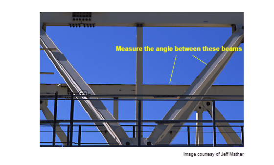
Step 1: Load Image

Read in gantrycrane.png and draw arrows pointing to two beams of interest. It is an image of a gantry crane used to assemble a bridge.

RGB = imread("gantrycrane.png");
imshow(RGB)

text(size(RGB,2),size(RGB,1)+15,"Image courtesy of Jeff Mather", ...
     FontSize=7,HorizontalAlignment="right");

line([300 328],[85 103],Color=[1 1 0]);
line([268 255],[85 140],Color=[1 1 0]);

text(150,72,"Measure the angle between these beams",Color="y", ...
     FontWeight="bold");

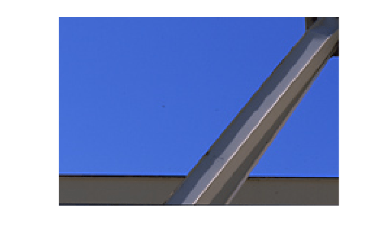
Step 2: Extract the Region of Interest

Crop the image to obtain only the beams of the gantry crane chosen earlier. This step will make it easier to extract the edges of the two metal beams.

You can obtain the coordinates of the rectangular region using pixel information displayed by imtool.

start_row = 34;
start_col = 208;

cropRGB = RGB(start_row:163,start_col:400,:);
imshow(cropRGB)

Store (x,y) offsets for later use; subtract 1 so that each offset will correspond to the last pixel before the region of interest.

offsetX = start_col-1;
offsetY = start_row-1;

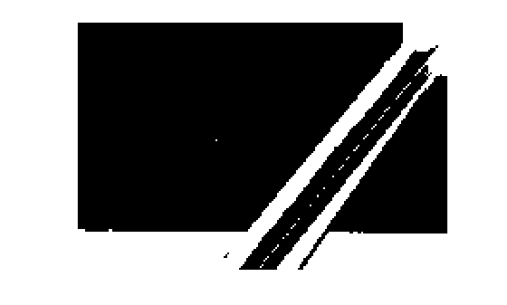
Step 3: Threshold the Image

The bwtraceboundary function expects objects of interest to be white in a binary image, so convert the image to black and white and take the image complement.

I = im2gray(cropRGB);
BW = imbinarize(I);
BW = ~BW;
imshow(BW)

Step 4: Find Initial Point on Each Boundary

The bwtraceboundary function requires that you specify a single point on a boundary. This point is used as the starting location for the boundary tracing process.

To extract the edge of the lower beam, pick a column in the image and inspect it until a transition from a background pixel to the object pixel occurs. Store this location for later use in bwtraceboundary routine. Repeat this procedure for the other beam, but this time tracing horizontally.

dim = size(BW);

% Horizontal beam
col1 = 4;
row1 = find(BW(:,col1), 1);

% Angled beam
row2 = 12;
col2 = find(BW(row2,:), 1);

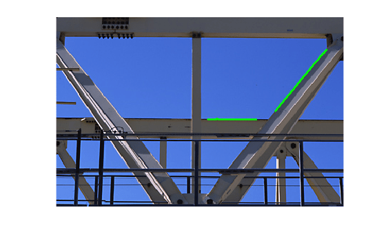
Step 5: Trace the Boundaries

The bwtraceboundary routine is used to extract (X, Y) locations of the boundary points. In order to maximize the accuracy of the angle and point of intersection calculations, it is important to extract as many points belonging to the beam edges as possible. You should determine the number of points experimentally. Since the initial point for the horizontal bar was obtained by scanning from north to south, it is safest to set the initial search step to point towards the outside of the object, i.e. "North".

boundary1 = bwtraceboundary(BW,[row1, col1],"N",8,70);

% Set the search direction to counterclockwise, in order to trace downward
boundary2 = bwtraceboundary(BW,[row2, col2],"E",8,90,"counter");

imshow(RGB)
hold on

% Apply offsets in order to draw in the original image
plot(offsetX+boundary1(:,2),offsetY+boundary1(:,1),"g",LineWidth=2);
plot(offsetX+boundary2(:,2),offsetY+boundary2(:,1),"g",LineWidth=2);

Step 6: Fit Lines to the Boundaries

Although (X,Y) coordinates pairs were obtained in the previous step, not all of the points lie exactly on a line. Which ones should be used to compute the angle and point of intersection? Assuming that all of the acquired points are equally important, fit lines to the boundary pixel locations.

The equation for a line is y = [x 1]*[a; b]. You can solve for parameters 'a' and 'b' in the least-squares sense by using polyfit.

ab1 = polyfit(boundary1(:,2),boundary1(:,1),1);
ab2 = polyfit(boundary2(:,2),boundary2(:,1),1);

Step 7: Find the Angle of Intersection

Use the dot product to find the angle.

vect1 = [1 ab1(1)]; % Create a vector based on the line equation
vect2 = [1 ab2(1)];
dp = dot(vect1, vect2);

Compute vector lengths

length1 = sqrt(sum(vect1.^2));
length2 = sqrt(sum(vect2.^2));

Obtain the larger angle of intersection in degrees

angle = 180-acos(dp/(length1*length2))*180/pi

angle = 129.4971

Step 8: Find the Point of Intersection

Solve the system of two equations in order to obtain (X,Y) coordinates of the intersection point.

intersection = [1 ,-ab1(1); 1, -ab2(1)] \ [ab1(2); ab2(2)];

Apply offsets in order to compute the location in the original uncropped image

intersection = intersection + [offsetY; offsetX]

intersection = 2×1

  143.0917
  295.7494

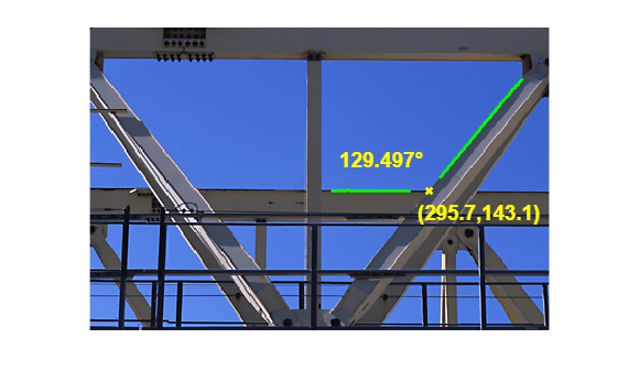
Step 9: Plot the Results

Draw an "X" at the point of intersection

inter_x = intersection(2);
inter_y = intersection(1);
plot(inter_x,inter_y,"yx","LineWidth",2);

Annotate the image with the angle between the beams and the (x,y) coordinates of the intersection point.

angleString = [sprintf("%1.3f",angle)+"{\circ}"];
text(inter_x-80,inter_y-25,angleString, ...
     Color="y",FontSize=14,FontWeight="bold");

intersectionString = sprintf("(%2.1f,%2.1f)",inter_x,inter_y);
text(inter_x-10,inter_y+20,intersectionString,...
     Color="y",FontSize=14,FontWeight="bold");