Log and Visualize 3-D Data from Velodyne LiDAR Sensor
This example shows how to acquire lidar data from a Velodyne LiDAR® sensor device. A lidar sensor creates a 3-D map of the surrounding environment by using scanning laser beams and time of flight distance measurements. Lidar systems are used in a variety of application areas, such as a 3-D mapping, surveying, industrial automation, and autonomous vehicle navigation.
A Velodyne Puck (VLP-16) sensor is used in this example. This model has 16 scanning laser beams (channels), up to 360 degrees horizontal field of view (FOV), 30 degrees vertical FOV, and 100 meter range. The velodyneLidar interface in MATLAB® supports a variety of Velodyne LiDAR models. Choose a sensor model appropriate for your particular application by consulting the instrument specifications provided by the manufacturer.
Requirements
This example requires:
MATLAB R2020b or later.
Lidar Toolbox™.
Lidar Toolbox Support Package for Velodyne LiDAR Sensors.
A supported Velodyne LiDAR sensor. A Velodyne Puck (VLP-16) is used in this example.
Set Up and Configure Velodyne LiDAR Sensor
The Velodyne Puck (VLP-16) sensor is an Ethernet network connected device that provides an integrated web server for configuring operating parameters, such as FOV or rotation rate. Consult the VLP-16 User Manual for required network setup and sensor parameter configuration. In this example, the VLP-16 sensor is directly connected to a computer with a dedicated Ethernet adapter, and the sensor's default IP address value is used (192.168.1.201).
To configure the sensor's parameters, access the sensor's web interface by opening the sensor's web server URL (http://192.168.1.201/) in a web browser. To test the sensor network setup, configuration, and operation, use VeloView, an application provided by the manufacturer.
Connect to Velodyne LiDAR Sensor
Create a velodynelidar object to receive data from the VLP-16 device. MATLAB uses the default UDP port value of 2368 to receive data from the device. If your device is configured to broadcast data to a different port, you need to specify the port number as an additional name-value pair argument, for example, velodynelidar('VLP16','Port',2368).
lidar = velodynelidar('VLP16');Preview Live Lidar Data
View live scan data acquired from the lidar sensor using the preview function.
preview(lidar)
pause(10)
closePreview(lidar)
Acquire Lidar Data
The lidar sensor continuously streams 3-D maps of the surroundings as frames of data. Each data frame represents one full scan of the FOV. The velodynelidar interface provides a continuous buffered acquisition functionality, which can be initiated using the start function. The processed lidar data frames are stored in an input buffer.
% Start acquisition
start(lidar)
Read one data frame from the lidar sensor. Each data frame is represented in MATLAB as a pointCloud datatype. The data values represent a distance measurement and the default units are meters (m).
Use the read function to read data frames into MATLAB workspace. You can use the optional second argument to read the frame timestamp. The timestamp is returned as a datetime datatype.
[frame,timestamp] = read(lidar,1)
frame =
  pointCloud with properties:

     Location: [32×1846×3 double]
        Color: []
       Normal: []
    Intensity: [32×1846 double]
        Count: 59072
      XLimits: [-90.9482 83.9612]
      YLimits: [-103.9809 102.8859]
      ZLimits: [-3.2730 15.8287]
timestamp = datetime
   24-Apr-2019 12:20:15:622
Visualize Acquired Data Frame
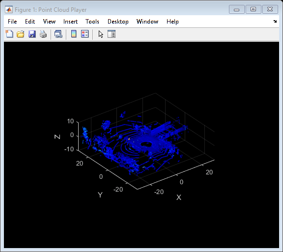
Display the data frame (point cloud) using pcplayer and use the data limits as the view XYZ limits.
lidarViewer = pcplayer(frame.XLimits,frame.YLimits,frame.ZLimits);
view(lidarViewer, frame)
Configure the viewing region of interest by setting the pcplayer axes limits.
lidarViewer.Axes.XLim = [-30 30];
lidarViewer.Axes.YLim = [-30 30];
lidarViewer.Axes.ZLim = [-10 10];

Read a Sequence of Frames
Read a sequence of 100 frames. The acquired frames data are represented as a pointCloud array, and the acquired timestamps as a datetime array.
numFrames = 100;
[frames,timestamps] = read(lidar,numFrames);
Stop Acquisition
Stop acquisition and disconnect from the lidar sensor.
stop(lidar)
clear lidar
Save Acquired Data
Save the acquired data frames and timestamps to a MAT file.
save lidardata.mat frames timestamps
Determine Lidar Frame Rate
You can use the timestamps data to determine the number of acquired lidar data frames per second (frame rate). The lidar sensor's frame rate depends on the configured motor RPM, FOV, and other sensor parameters.
fps = 1/mean(seconds(diff(timestamps)))
fps = 11.6484
View Replay of Lidar Data
Use the existing pcplayer object (lidarViewer) to replay acquired frames as an animation. This uses a custom helper function (replay), which is included at the end of this example.
replay(lidarViewer,frames,fps)

Lidar Data Processing and Analysis
The following toolboxes provide specialized algorithms and tools for processing and analysis of lidar and 3-D point cloud data:
Computer Vision Toolbox™
Automated Driving Toolbox™
Local Functions
function replay(lidarViewer,frames,fps)
%REPLAY Replays point cloud array data in a PCPLAYER figure
% LIDARVIEWER is an existing PCPLAYER object
% FRAMES is a pointCloud array
% FPS is the approximate playback frame rate
%
% Example usage:
%  lidar = velodynelidar('VLP16');
%  start(lidar)
%  [frames,timestamps] = read(lidar,100);
%  stop(lidar)
%  clear lidar
%  fps = 1/mean(seconds(diff(timestamps)));
%  lidarViewer = pcplayer([-40 40], [-40 40],[-10 10]);
%  replay(lidarViewer,frames,fps);

    dt = 1/fps;

    for ii = 1:numel(frames)
        view(lidarViewer,frames(ii))
        pause(dt)
    end

end
See Also
velodynelidar | preview | read | start | stop | pcplayer