Roots of Scalar Functions
Solving a Nonlinear Equation in One Variable
The fzero function attempts to find a root of one equation with one variable. You can call this function with either a one-element starting point or a two-element vector that designates a starting interval. If you give fzero a starting point x0, fzero first searches for an interval around this point where the function changes sign. If the interval is found, fzero returns a value near where the function changes sign. If no such interval is found, fzero returns NaN. Alternatively, if you know two points where the function value differs in sign, you can specify this starting interval using a two-element vector; fzero is guaranteed to narrow down the interval and return a value near a sign change.
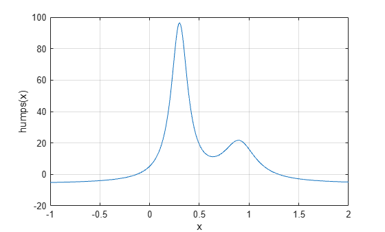
The following sections contain two examples that illustrate how to find a zero of a function using a starting interval and a starting point. The examples use the function humps.m, which is provided with MATLAB®. The following figure shows the graph of humps.
x = -1:.01:2;
y = humps(x);
plot(x,y)
xlabel('x');
ylabel('humps(x)')
grid on
Setting Options for fzero
You can control several aspects of the fzero function by setting options. You set options using optimset. Options include:
Choosing the amount of display
fzerogenerates — see Set Optimization Options, Using a Starting Interval, and Using a Starting Point.Choosing various tolerances that control how
fzerodetermines it is at a root — see Set Optimization Options.Choosing a plot function for observing the progress of
fzerotowards a root — see Optimization Solver Plot Functions.Using a custom-programmed output function for observing the progress of
fzerotowards a root — see Optimization Solver Output Functions.
Using a Starting Interval
The graph of humps indicates that the function is negative at x = -1 and positive at x = 1. You can confirm this by calculating humps at these two points.
humps(1)
ans =
16
humps(-1)
ans =
-5.1378
Consequently, you can use [-1 1] as a starting interval for fzero.
The iterative algorithm for fzero finds smaller and smaller subintervals of [-1 1]. For each subinterval, the sign of humps differs at the two endpoints. As the endpoints of the subintervals get closer and closer, they converge to zero for humps.
To show the progress of fzero at each iteration, set the Display option to iter using the optimset function.
options = optimset('Display','iter');
Then call fzero as follows:
a = fzero(@humps,[-1 1],options)
 Func-count    x          f(x)             Procedure
    2              -1      -5.13779        initial
    3       -0.513876      -4.02235        interpolation
    4       -0.513876      -4.02235        bisection
    5       -0.473635      -3.83767        interpolation
    6       -0.115287      0.414441        bisection
    7       -0.115287      0.414441        interpolation
    8       -0.132562    -0.0226907        interpolation
    9       -0.131666    -0.0011492        interpolation
   10       -0.131618   1.88371e-07        interpolation
   11       -0.131618   -2.7935e-11        interpolation
   12       -0.131618   8.88178e-16        interpolation
   13       -0.131618   8.88178e-16        interpolation

Zero found in the interval [-1, 1]
a =
-0.1316
Each value x represents the best endpoint so far. The Procedure column tells you whether each step of the algorithm uses bisection or interpolation.
You can verify that the function value at a is close to zero by entering
humps(a)
ans =
8.8818e-16
Using a Starting Point
Suppose you do not know two points at which the function values of humps differ in sign. In that case, you can choose a scalar x0 as the starting point for fzero. fzero first searches for an interval around this point on which the function changes sign. If fzero finds such an interval, it proceeds with the algorithm described in the previous section. If no such interval is found, fzero returns NaN.
For example, set the starting point to -0.2, the Display option to Iter, and call fzero:
options = optimset('Display','iter');
a = fzero(@humps,-0.2,options)
Search for an interval around -0.2 containing a sign change:
 Func-count    a          f(a)             b          f(b)        Procedure
    1            -0.2      -1.35385          -0.2      -1.35385   initial interval
    3       -0.194343      -1.26077     -0.205657      -1.44411   search
    5          -0.192      -1.22137        -0.208       -1.4807   search
    7       -0.188686      -1.16477     -0.211314      -1.53167   search
    9          -0.184      -1.08293        -0.216      -1.60224   search
   11       -0.177373     -0.963455     -0.222627      -1.69911   search
   13          -0.168     -0.786636        -0.232      -1.83055   search
   15       -0.154745      -0.51962     -0.245255      -2.00602   search
   17          -0.136     -0.104165        -0.264      -2.23521   search
   18        -0.10949      0.572246        -0.264      -2.23521   search

Search for a zero in the interval [-0.10949, -0.264]:
 Func-count    x          f(x)             Procedure
   18        -0.10949      0.572246        initial
   19       -0.140984     -0.219277        interpolation
   20       -0.132259    -0.0154224        interpolation
   21       -0.131617   3.40729e-05        interpolation
   22       -0.131618  -6.79505e-08        interpolation
   23       -0.131618  -2.98428e-13        interpolation
   24       -0.131618   8.88178e-16        interpolation
   25       -0.131618   8.88178e-16        interpolation

Zero found in the interval [-0.10949, -0.264]
a =
-0.1316
The endpoints of the current subinterval at each iteration are listed under the headings a and b, while the corresponding values of humps at the endpoints are listed under f(a) and f(b), respectively.
Note: The endpoints a and b are not listed in any specific order: a can be greater than b or less than b.
For the first nine steps, the sign of humps is negative at both endpoints of the current subinterval, which is shown in the output. At the tenth step, the sign of humps is positive at a, -0.10949, but negative at b, -0.264. From this point on, the algorithm continues to narrow down the interval [-0.10949 -0.264], as described in the previous section, until it reaches the value -0.1316.
See Also
Topics
- Roots of Polynomials
- Optimizing Nonlinear Functions
- Systems of Nonlinear Equations (Optimization Toolbox)