besselh

Bessel function of third kind (Hankel function)

Syntax

H = besselh(nu,Z)

H = besselh(nu,K,Z)

H = besselh(nu,K,Z,scale)

Description

H = besselh(nu,Z) computes the Hankel function of the first kind $$H_{\nu }^{\left(1\right)}\left(z\right)=J_{\nu }\left(z\right)+i{Y}_{\nu }\left(z\right)$$ for each element in array Z.

H = besselh(nu,K,Z) computes the Hankel function of the first or second kind $$H_{\nu }{}^{\left(K\right)}\left(z\right)$$, where K is 1 or 2, for each element of array Z.

H = besselh(nu,K,Z,scale) specifies whether to scale the Hankel function to avoid overflow or loss of accuracy. If scale is 1, then Hankel functions of the first kind $$H_{\nu }^{\left(1\right)}\left(z\right)$$ are scaled by $$e^{-iZ}$$, and Hankel functions of the second kind $$H_{\nu }^{\left(2\right)}\left(z\right)$$ are scaled by $$e^{+iZ}$$.

Examples

Modulus and Phase of Hankel Function

Generate the contour plots of the modulus and phase of the Hankel function $$H_0^{(1)}(z)$$ [1].

Create a grid of values for the domain.

[X,Y] = meshgrid(-4:0.002:2,-1.5:0.002:1.5);

Calculate the Hankel function over this domain and generate the modulus contour plot.

H = besselh(0,X+1i*Y);
contour(X,Y,abs(H),0:0.2:3.2)
hold on

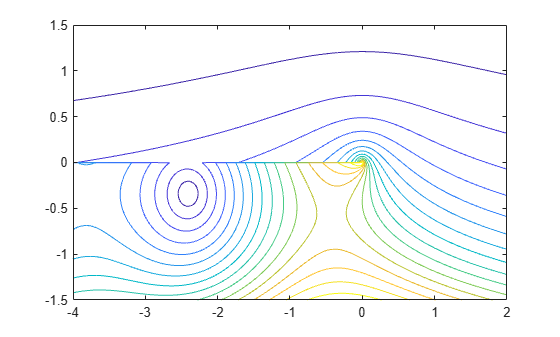
In the same figure, add the contour plot of the phase.

contour(X,Y,rad2deg(angle(H)),-180:10:180)
hold off

Asymptotic Behavior

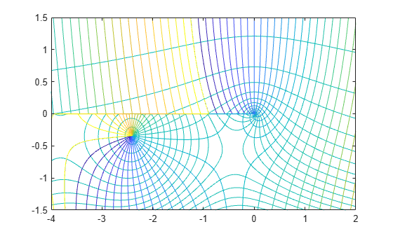
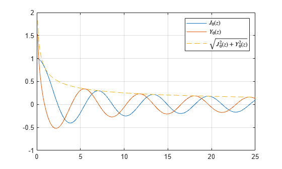
Plot the real and imaginary parts of the Hankel function of the second kind and examine their asymptotic behavior.

Calculate the Hankel function of the second kind ${\mathit{H}}_0^{\left(2\right)}\left(\mathit{z}\right)={\mathit{J}}_0\left(\mathit{z}\right)-\mathit{i}{\mathit{Y}}_0\left(\mathit{z}\right)$ in the interval $\left[0.1,25\right]$.

k = 2;
nu = 0;
z = linspace(0.1,25,200);
H = besselh(nu,k,z);

Plot the real and imaginary parts of the function. In the same figure, plot the linear combination $\sqrt{{\mathit{J}}_0^2\left(\mathit{z}\right)+{\mathit{Y}}_0^2\left(\mathit{z}\right)}$, which reveals the asymptotic behavior of the magnitudes of the real and imaginary parts.

plot(z,real(H),z,imag(H))
grid on
hold on
M = sqrt(real(H).^2 + imag(H).^2);
plot(z,M,'--')
legend('$J_0(z)$', '$Y_0(z)$', '$\sqrt{J_0^2 (z) + Y_0^2 (z)}$','interpreter','latex')

Exponentially Scaled Hankel Function

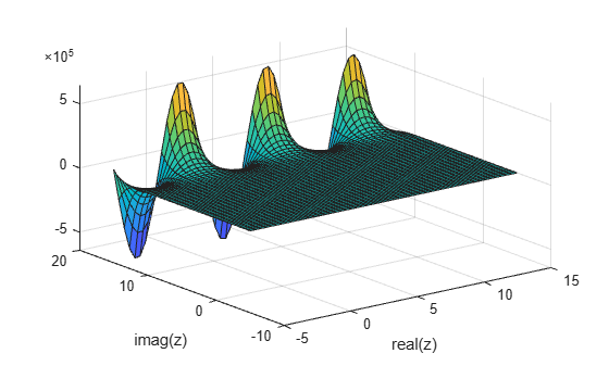
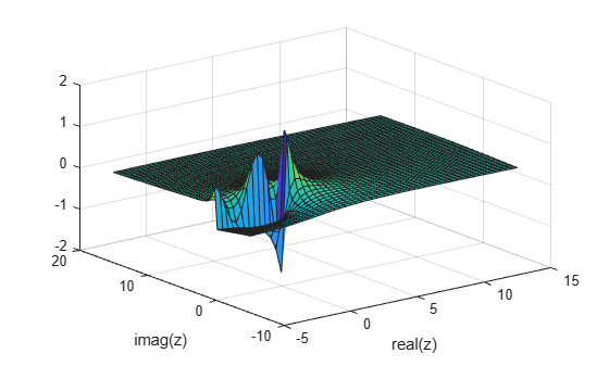
Calculate the exponentially scaled Hankel function ${\mathit{H}}_1^{\left(2\right)}\left(\mathit{z}\right){\cdot \mathit{e}}^{\mathrm{iz}}$ on the complex plane and compare it to the unscaled function.

Calculate the unscaled Hankel function of the second order on the complex plane. When z has a large positive imaginary part, the value of the function quickly diverges. This phenomenon limits the range of computable values.

k = 2;
nu = 1;
x = -5:0.4:15;
y = x';
z = x + 1i*y;
scaled = 1;
H = besselh(nu,k,z);
surf(x,y,imag(H))
xlabel('real(z)')
ylabel('imag(z)')

Now, calculate ${\mathit{H}}_1^{\left(2\right)}\left(\mathit{z}\right){\cdot \mathit{e}}^{\mathrm{iz}}$ on the complex plane and compare it to the unscaled function. The scaled function increases the range of computable values by avoiding overflow and loss of accuracy when z has a large positive imaginary part.

Hs = besselh(nu,k,z,scaled);
surf(x,y,imag(Hs))
xlabel('real(z)')
ylabel('imag(z)')

Input Arguments

nu — Equation order

scalar | vector | matrix | multidimensional array

Equation order, specified as a scalar, vector, matrix, or multidimensional array. nu specifies the order of the Hankel function. nu and Z must be the same size, or one of them can be scalar.

Example: besselh(3,Z)

Data Types: single | double

K — Kind of Hankel function

1 (default) | 2

Kind of Hankel function, specified as 1 or 2.

• If K = 1, then besselh computes the Hankel function of the first kind $$H_{\nu }^{\left(1\right)}\left(z\right)=J_{\nu }\left(z\right)+i{Y}_{\nu }\left(z\right)$$.

• If K = 2, then besselh computes the Hankel function of the second kind $$H_{\nu }^{\left(2\right)}\left(z\right)=J_{\nu }\left(z\right)-i{Y}_{\nu }\left(z\right)$$.

Example: besselh(nu,2,Z)

Z — Functional domain

scalar | vector | matrix | multidimensional array

Functional domain, specified as a scalar, vector, matrix, or multidimensional array. nu and Z must be the same size, or one of them can be scalar.

Example: besselh(nu,[1-1i 1+0i 1+1i])

Data Types: single | double
Complex Number Support: Yes

scale — Toggle to scale function

0 (default) | 1

Toggle to scale function, specified as one of these values:

• 0 (default) — No scaling

• 1 — Scale the output of besselh, depending on the value of K:

  • If K = 1, then scale the Hankel function of the first kind $$H_{\nu }^{\left(1\right)}\left(z\right)$$ by $$e^{-iZ}$$.

  • If K = 2, then scale Hankel function of the second kind $$H_{\nu }^{\left(2\right)}\left(z\right)$$ by $$e^{+iZ}$$.

  On the complex plane, $$H_{\nu }^{\left(1\right)}\left(z\right)$$ overflows when imag(Z) is large and negative. Similarly, $$H_{\nu }^{\left(2\right)}\left(z\right)$$ overflows when imag(Z) is large and positive. Exponentially scaling the output of besselh is useful in these two cases since the function otherwise quickly loses accuracy or overflows the limits of double precision.

Example: besselh(nu,K,Z,1)

More About

Hankel Functions and Bessel’s Equation

This differential equation, where ν is a real constant, is called Bessel's equation:

$$z^2\frac{d^{2}y}{d{z}^2}+z\frac{dy}{dz}+\left(z^2-{\nu }^2\right)y=0.$$

Its solutions are known as Bessel functions.

The Bessel functions of the first kind, denoted J_ν(z) and J_–ν(z), form a fundamental set of solutions of Bessel's equation for noninteger ν. The Bessel functions of the second kind, denoted Y_ν(z), form a second solution of Bessel's equation—linearly independent of J_ν(z)—defined by

$$Y_{\nu }(z)=\frac{J_{\nu }(z)\cos (\nu \pi )-J_{-\nu }(z)}{\sin (\nu \pi )}.$$

The Bessel functions of the third kind, also called Hankel functions of the first and second kind, are defined by linear combinations of the Bessel functions, where J_ν(z) is besselj, and Y_ν(z) is bessely:

$$\begin{array}{l}{H}_{\nu }^{(1)}(z)=J_{\nu }(z)+i{Y}_{\nu }(z)\\ H_{\nu }^{(2)}(z)=J_{\nu }(z)-i{Y}_{\nu }(z).\end{array}$$

References

[1] Abramowitz, M., and I.A. Stegun. Handbook of Mathematical Functions. National Bureau of Standards, Applied Math. Series #55, Dover Publications, 1965.

Extended Capabilities

Tall Arrays

Calculate with arrays that have more rows than fit in memory.

This function fully supports tall arrays. For more information, see Tall Arrays.

C/C++ Code Generation

Generate C and C++ code using MATLAB® Coder™.

Usage notes and limitations:

• Always returns a complex result.

• Strict single-precision calculations are not supported. In the generated code, single-precision inputs produce single-precision outputs. However, variables inside the function might be double-precision.

GPU Code Generation

Generate CUDA® code for NVIDIA® GPUs using GPU Coder™.

Usage notes and limitations:

• Always returns a complex result.

• Strict single-precision calculations are not supported. In the generated code, single-precision inputs produce single-precision outputs. However, variables inside the function might be double-precision.

Thread-Based Environment

Run code in the background using MATLAB® backgroundPool or accelerate code with Parallel Computing Toolbox™ ThreadPool.

This function fully supports thread-based environments. For more information, see Run MATLAB Functions in Thread-Based Environment.

Distributed Arrays

Partition large arrays across the combined memory of your cluster using Parallel Computing Toolbox™.

This function fully supports distributed arrays. For more information, see Run MATLAB Functions with Distributed Arrays (Parallel Computing Toolbox).

Version History

Introduced before R2006a