setInitialConditions
Give initial conditions or initial solution
Syntax
Description
setInitialConditions(___,
sets initial conditions on a geometry region using any of the arguments in the
previous syntaxes.RegionType,RegionID)
ic = setInitialConditions(___)
Examples
Create a PDE model, import geometry, and set the initial condition to 50 on the entire geometry.
model = createpde();
importGeometry(model,"BracketWithHole.stl");
setInitialConditions(model,50);Set different initial conditions for each component of a system of PDEs.
Create a PDE model for a system with five components. Import the Block.stl geometry.
model = createpde(5);
importGeometry(model,"Block.stl");
Set the initial conditions for each component to twice the component number.
u0 = [2:2:10]';
setInitialConditions(model,u0)
ans =
  GeometricInitialConditions with properties:

           RegionType: 'cell'
             RegionID: 1
         InitialValue: [5×1 double]
    InitialDerivative: []
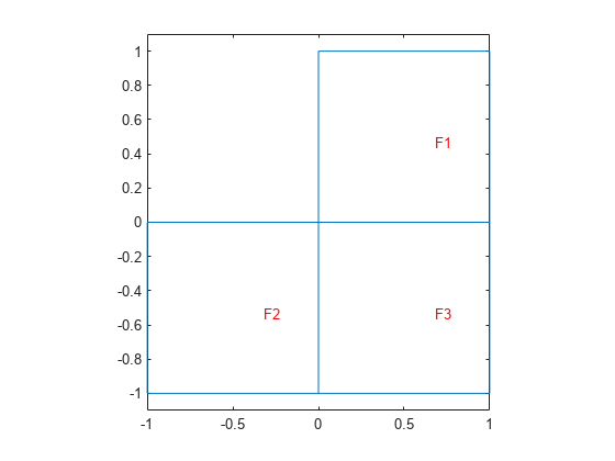
Set different initial conditions on each portion of the L-shaped membrane geometry.
Create a model, set the geometry function, and view the subdomain labels.
model = createpde();
geometryFromEdges(model,@lshapeg);
pdegplot(model,"FaceLabels","on")
axis equal
ylim([-1.1,1.1])

Set subdomain 1 to initial value -1, subdomain 2 to initial value 1, and subdomain 3 to initial value 5.
setInitialConditions(model,-1);
setInitialConditions(model,1,"Face",2);
setInitialConditions(model,5,"Face",3);
The initial setting applies to the entire geometry. The subsequent settings override the initial settings for regions 2 and 3.
Set initial conditions for the L-shaped membrane geometry to be , except in the lower left square where it is .
model = createpde();
geometryFromEdges(model,@lshapeg);
pdegplot(model,"FaceLabels","on")
axis equal
ylim([-1.1,1.1])
Set the initial conditions to .
initfun = @(location)location.x.^2 + location.y.^2;
setInitialConditions(model,initfun);
Set the initial conditions on region 2 to . This setting overrides the first setting because you apply it after the first setting.
initfun2 = @(location)location.x.^2 - location.y.^4;
setInitialConditions(model,initfun2,"Face",2);Hyperbolic equations have nonzero m coefficient, so you must set both the u0 and ut0 arguments.
Import the Block.stl to a PDE model with N = 3 components.
model = createpde(3);
importGeometry(model,"Block.stl");
Set the initial condition value to be 0 for all components. Set the initial derivative.
To create this initial gradient, write a function file, and ensure that the function is on your MATLAB® path.
function ut0 = ut0fun(location)
M = length(location.x);
ut0 = zeros(3,M);
denom = location.x.^2+location.y.^2+location.z.^2;
ut0(1,:) = 4 + location.x./denom;
ut0(2,:) = 5 - tanh(location.z);
ut0(3,:) = 10*location.y./denom;
end
Set the initial conditions.
setInitialConditions(model,0,@ut0fun)
ans =
  GeometricInitialConditions with properties:

           RegionType: 'cell'
             RegionID: 1
         InitialValue: 0
    InitialDerivative: @ut0fun
Set initial conditions using the solution from a previous analysis on the same geometry and mesh.
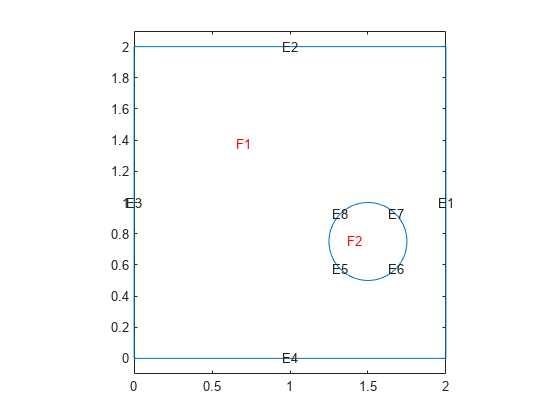
Create and view the geometry: a square with a circular subdomain.
% Square centered at (1,1), circle centered at (1.5,0.5).
rect1 = [3;4;0;2;2;0;0;0;2;2];
circ1 = [1;1.5;.75;0.25];
% Append extra zeros to the circle;
circ1 = [circ1;zeros(length(rect1)-length(circ1),1)];
gd = [rect1,circ1];
ns = char('rect1','circ1');
ns = ns';
sf = 'rect1+circ1';
[dl,bt] = decsg(gd,sf,ns);
pdegplot(dl,"EdgeLabels","on","FaceLabels","on")
axis equal
ylim([-0.1,2.1])
Include the geometry in a PDE model, set boundary and initial conditions, and specify coefficients.
model = createpde();
geometryFromEdges(model,dl);

% Set boundary conditions that the upper
% and left edges are at temperature 10.
applyBoundaryCondition(model,"dirichlet", ...
                             "Edge",[2,3],"u",10);

% Set initial conditions that the square region
% is at temperature 0,
% and the circle is at temperature 100.
setInitialConditions(model,0);
setInitialConditions(model,100,"Face",2);

specifyCoefficients(model,"m",0,...
                          "d",1,...
                          "c",1,...
                          "a",0,...
                          "f",0);
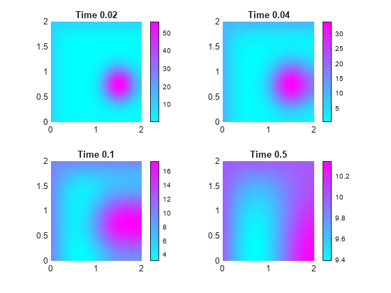
Solve the problem for times 0 through 1/2 in steps of 0.01.
generateMesh(model,"Hmax",0.05);
tlist = 0:0.01:0.5;
results = solvepde(model,tlist);
Plot the solution for times 0.02, 0.04, 0.1, and 0.5.
sol = results.NodalSolution;

subplot(2,2,1)
pdeplot(model,"XYData",sol(:,3))
title("Time 0.02")
subplot(2,2,2)
pdeplot(model,"XYData",sol(:,5))
title("Time 0.04")
subplot(2,2,3)
pdeplot(model,"XYData",sol(:,11))
title("Time 0.1")
subplot(2,2,4)
pdeplot(model,"XYData",sol(:,51))
title("Time 0.5")
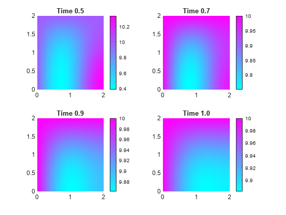
Now, resume the analysis and solve the problem for times from 1/2 to 1. Use the previously obtained solution for time 1/2 as an initial condition. Since 1/2 is the last element in tlist, you do not need to specify the solution time index. By default, setInitialConditions uses the last solution index.
setInitialConditions(model,results)
ans =
  NodalInitialConditions with properties:

         InitialValue: [7385×1 double]
    InitialDerivative: []
Solve the problem for times 1/2 through 1 in steps of 0.01.
tlist1 = 0.5:0.01:1.0;
results1 = solvepde(model,tlist1);
Plot the solution for times 0.5, 0.7, 0.9, and 1.
sol1 = results1.NodalSolution;

figure

subplot(2,2,1)
pdeplot(model,"XYData",sol1(:,1))
title("Time 0.5")
subplot(2,2,2)
pdeplot(model,"XYData",sol1(:,21))
title("Time 0.7")
subplot(2,2,3)
pdeplot(model,"XYData",sol1(:,41))
title("Time 0.9")
subplot(2,2,4)
pdeplot(model,"XYData",sol1(:,51))
title("Time 1.0")
To use the previously obtained solution for a particular solution time instead of the last one, specify the solution time index as a third parameter of setInitialConditions. For example, use the solution at time 0.2, which is the 21st element in tlist.
setInitialConditions(model,results,21)
ans =
  NodalInitialConditions with properties:

         InitialValue: [7385×1 double]
    InitialDerivative: []
Solve the problem for times 0.2 through 1 in steps of 0.01.
tlist2 = 0.2:0.01:1.0;
results2 = solvepde(model,tlist2);
Input Arguments
Output Arguments
Tips
To ensure that the model has the correct
TimeDependentproperty setting, if possible specify coefficients before setting initial conditions.To avoid assigning initial conditions to a wrong region, ensure that you are using the correct geometric region IDs by plotting and visually inspecting the geometry.