phased.NonlinearFMWaveform
Description
The phased.NonlinearFMWaveform
System object™ creates a frequency-modulated waveform whose frequency is a nonlinear function
of time (NLFM). NLFM waveforms achieve low-range sidelobes by shaping the spectrum using
frequency modulation. Four different waveforms are supported depending on the
FrequencyModulation property:
'Polynomial'– Generate a waveform with an instantaneous frequency that follows a polynomial function.'Hyperbolic'– Generate a hyperbolic frequency modulated (HFM) waveform.'Hybrid Linear-Tangent'– Generate a hybrid NLFM waveform that combines an LFM waveform with tan-FM waveform.'Stepped Price'– Generate a stepped version of Price's NLFM waveform.
To create the waveforms:
Create the
phased.NonlinearFMWaveformobject and set its properties.Call the object with arguments, as if it were a function.
To learn more about how System objects work, see What Are System Objects?
Creation
Description
waveform = phased.NonlinearFMWaveformwaveform
System object. By default, the waveform has a polynomial frequency modulation.
waveform = phased.NonlinearFMWaveform(Name = Value)waveform
System object with each specified property Name set to the specified
Value. You can specify additional name-value pair arguments in any
order as (Name1 =
Value1,...,NameN =
ValueN).
Properties
Usage
Syntax
Description
Y = waveform()Y. Y can
contain either a certain number of pulses or a certain number of samples.
Y = waveform(prfidx)prfidx.
The index identifies the entries specified in the PRF property. This
syntax applies when you set the PRFSelectionInputPort property to
true.
Use this syntax for the cases where the transmitted pulse needs to be dynamically
selected. In such situations, the PRF property includes a list of
predetermined choices of PRF's. During the simulation, using prfidx,
one of the PRFs is selected as the PRF for the next transmission.
Note that the transmission always finishes the current pulse before starting the next
pulse. Therefore, when you set the OutputFormat property to
'Samples' and then specify the NumSamples
property to be shorter than a pulse, it is possible that during a given simulation step,
if the entire output is needed to finish the previously transmitted pulse, the specified
prfidx is ignored.
Y = waveform(freqoffset)freqoffset as a finite
real value. The offset is used to generate the waveform with a frequency offset. Use this
syntax for the cases where the transmit pulse frequency needs to be dynamically updated.
To enable this syntax set the FrequencyOffsetSource property to
'Input port'.
[
also returns the current pulse repetition frequency, Y,PRF] = waveform(___)PRF. To enable
this syntax, set the PRFOutputPort property to
true and set the OutputFormat property to
'Pulses'.
[
returns an additional output Y,coeff]= waveform()coeff, as the matched filter
coefficients. To use this syntax, set the CoefficientsOutputPort
property to true.
You can combine optional input and output arguments when their enabling properties are set. Optional inputs and outputs must be listed in the same order as the order of the enabling properties. For example,
[Y,PRF,coeff] = waveform(prfidx,freqoffset)
Input Arguments
Output Arguments
Object Functions
To use an object function, specify the
System object as the first input argument. For
example, to release system resources of a System object named obj, use
this syntax:
release(obj)
Examples
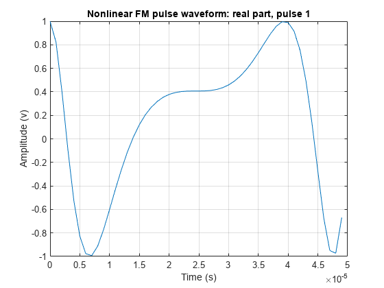
Create a nonlinear FM waveform with the default polynomial frequency modulation.
waveform = phased.NonlinearFMWaveform()
waveform =
  phased.NonlinearFMWaveform with properties:

                SampleRate: 1000000
     DurationSpecification: 'Pulse width'
                PulseWidth: 5.0000e-05
                       PRF: 10000
     PRFSelectionInputPort: false
       FrequencyModulation: 'Polynomial'
    PolynomialCoefficients: [1 0 0]
            SweepBandwidth: 100000
             SweepInterval: 'Positive'
                  Envelope: 'Rectangular'
     FrequencyOffsetSource: 'Property'
           FrequencyOffset: 0
              OutputFormat: 'Pulses'
                 NumPulses: 1
             PRFOutputPort: false
    CoefficientsOutputPort: false
Display the real part of the waveform.
plot(waveform)
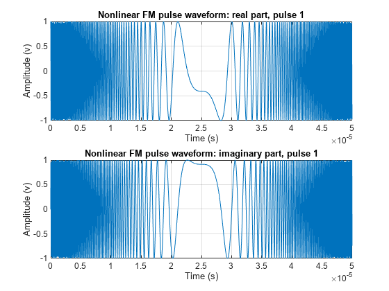
Create and plot a quadratic FM pulse waveform. The pulse has a 10 MHz bandwidth and 50 sec duration. The pulse sample rate is 10 times the bandwidth.
BW = 10e6;
T = 50e-6;
waveform = phased.NonlinearFMWaveform( ...
    'SampleRate',10*BW,'SweepBandwidth',BW, ...
    'PulseWidth',T);
plot(waveform,PlotType='complex')
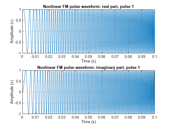
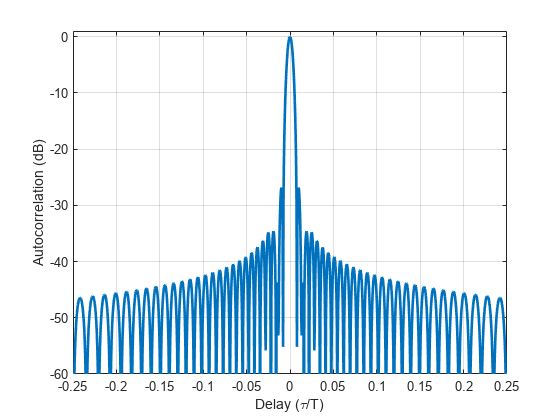
Generate samples of a hybrid linear-tangent FM waveform with a bandwidth of 2 kHz and a pulse width of 100 ms. Set the pulse repetition frequency to 5 Hz and the sample frequency to 20 kHz. Set the factor controlling the balance between the linear and the nonlinear terms to 0.5. Set the factor controlling the portion of the tan(x) curve used for frequency modulation to 1.4. Plot the autocorrelation function to determine the resulting range sidelobe level.
BW = 2000;
T = 100e-3;
PRF = 5;
fs = 10*BW;
Set the balance between tan-FM and LFM to 0.5 and set the portion of tan(x) to use to 1.4.
alpha = 0.5;
gamma = 1.4;
Create the waveform and plot the real and imaginary parts.
waveform = phased.NonlinearFMWaveform('SampleRate',fs,'PulseWidth',T, ...
    'PRF',PRF,'FrequencyModulation','Hybrid Linear-Tangent', ...
    'LinearTangentBalance',alpha,'TangentCurvePortion',gamma, ...
    'SweepBandwidth',BW,'OutputFormat','Pulses','NumPulses',2);
wav = waveform();
figure
plot(waveform,PlotType='complex')
Compute and plot the autocorrelation function.
[acf,delay] = ambgfun(wav,waveform.SampleRate,waveform.PRF, ...
    Cut='Doppler');
figure
plot(delay/waveform.PulseWidth,mag2db(acf),LineWidth=2)
grid on
xlim([-0.25 0.25])
ylim([-60 1])
xlabel('Delay (\tau/T)')
ylabel('Autocorrelation (dB)')
Generate output samples of a nonlinear FM pulse waveform based on the stepped version of Price's waveform. The pulse width is 5e-6 seconds. The waveform performs 50 frequency steps within one pulse. The time-bandwidth products of the linear and nonlinear components are 20 and 40 respectively. The start frequency of the sweep is 15 MHz. Generate matched filter coefficients and then apply the matched filter.
T = 5e-6;
M = 50;
BLT = 20;
BCT = 40;
bfs = [BLT BCT]/T;
fs = 100e6;
fstart = 15e6;

waveform = phased.NonlinearFMWaveform(SampleRate=fs, ...
    PulseWidth=T,FrequencyModulation='Stepped Price', ...
    BandwidthFactors=bfs,NumSteps=M,FrequencyOffset=fstart, ...
    OutputFormat='Pulses',CoefficientsOutputPort=true);
Plot the complex waveform.
figure
plot(waveform,PlotType='complex')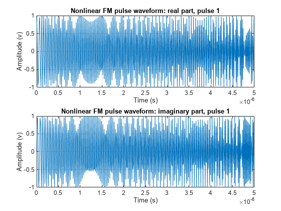
Obtain the resulting sweep bandwidth (Hz)
bandwidth(waveform)
ans =
4.3317e+07
Find the matched filter coefficients. Then plot the filtered waveform.
[wav,coeff] = waveform();
mf = phased.MatchedFilter(CoefficientsSource='Input port');
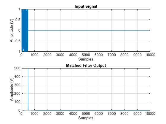
mfout = mf(wav,coeff);Plot the filter input and output.
figure
subplot(211)
plot(real(wav))
grid on
xlabel('Samples')
ylabel('Amplitude (V)')
title('Input Signal')

subplot(212)
plot(abs(mfout));
grid on
xlabel('Samples')
ylabel('Amplitude (V)')
title('Matched Filter Output')
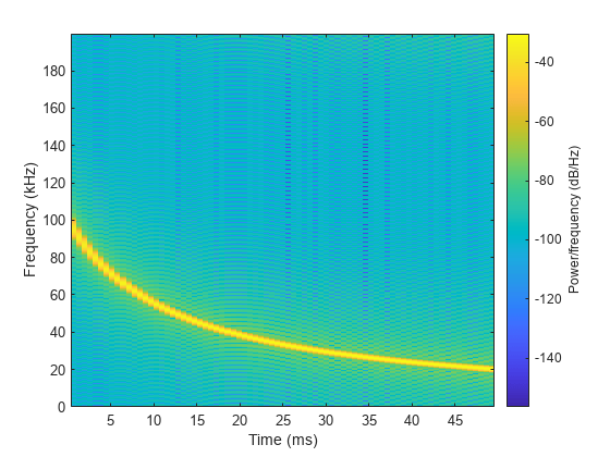
Create a hyperbolic frequency modulated (HFM) waveform. The start and the stop frequencies of the sweep are 100 kHz and 20 kHz, respectively. The pulse width is 50 ms. The sample rate is 200 kHz. Plot the spectrogram.
f1 = 100e3;
f2 = 20e3;
BW = f1 - f2;
T = 50e-3;
fs = 2*f1;
Create a hyperbolic FM waveform.
waveform = phased.NonlinearFMWaveform( ...
    SampleRate=fs,PulseWidth=T,SweepBandwidth=BW, ...
    FrequencyModulation='Hyperbolic', ...
    HyperbolicStartFrequency=f1, ...
    SweepDirection='down',PRF=1/T);
sig = waveform();
spectrogram(sig, 256, 128, 1024, fs, 'yaxis')
References
[1] Collins, T., and P. Atkins. "Nonlinear frequency modulation chirps for active sonar." IEE Proceedings-Radar, Sonar and Navigation 146.6 (1999): 312-316.
[2] Levanon, Nadav, and Eli Mozeson. Radar signals. John Wiley & Sons, 2004, pp. 92-93.
[3] Doerry, Armin Walter. "Generating nonlinear FM chirp waveforms for radar". No. SAND2006-5856. Sandia National Laboratories (SNL), Albuquerque, NM, and Livermore, CA (United States), 2006.
[4] Cook, C. E. "A class of nonlinear FM pulse compression signals." Proceedings of the IEEE 52.11 (1964): 1369-1371.
[5] Yang, J., and T. K. Sarkar. "Doppler‐invariant property of hyperbolic frequency modulated waveforms." Microwave and optical technology letters 48.6 (2006): 1174-1179.
[6] Melvin, William L., and James Scheer. Principles of modern radar: advanced techniques. SciTech Pub., 2013.
[7] Alphonse, Sebastian, and Geoffrey A. Williamson. "Evaluation of a class of NLFM radar signals." EURASIP Journal on Advances in Signal Processing 2019.1 (2019): 1-12.
Extended Capabilities
Version History
Introduced in R2023a