Accelerate Fault Diagnosis Using GPU Data Preprocessing and Deep Learning
This example shows how to use GPU computing to accelerate data preprocessing and deep learning for predictive maintenance workflows.
One of the easiest ways to speed up your code is to run it on a GPU, and many functions in MATLAB® automatically run on a GPU if you supply a gpuArray data argument. Starting from the code in the Rolling Element Bearing Fault Diagnosis Using Deep Learning example, this example demonstrates how to speed up execution in a predictive maintenance deep learning workflow by modifying it to run on a GPU. You can use a similar approach to accelerate many of your predictive maintenance workflows.
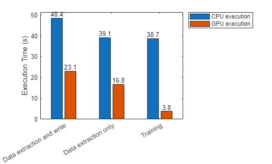
As this figure shows, you can significantly speed up data extraction and network training using a GPU.
Check GPU Support
Using a GPU requires Parallel Computing Toolbox™ and a supported GPU device. For information on supported devices, see GPU Computing Requirements (Parallel Computing Toolbox).
Check whether you have a supported GPU.
gpu = gpuDevice;
disp(gpu.Name + " GPU selected.")
NVIDIA RTX A5000 GPU selected.
If a function supports GPU array input, the documentation page for that function lists GPU support in the Extended Capabilities section. You can also filter lists of functions in the documentation to show only functions that support GPU array input. For more information, see Run MATLAB Functions on a GPU (Parallel Computing Toolbox).
After checking that you have a supported GPU, you follow the same steps as the previous example, with minor modifications to send data to the GPU and run functions on the GPU where possible. The code requires very little modification to run on a GPU.
The following figure shows a rolling element striking a local fault at the inner race. A common problem is detecting and identifying these faults.
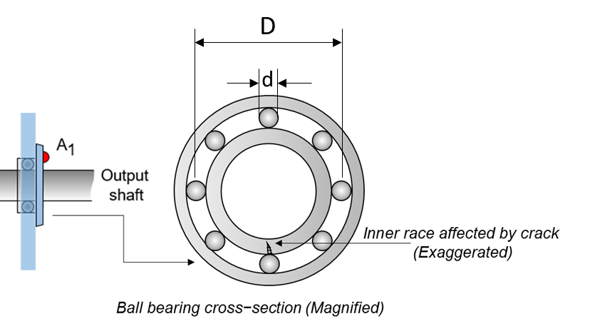
This example shows how to perform fault diagnosis of a rolling element bearing using a deep learning approach. The example demonstrates how to classify bearing faults by converting 1-D bearing vibration signals to 2-D images of scalograms and applying transfer learning using a pretrained network. Transfer learning significantly reduces the time spent on feature extraction and feature selection in conventional bearing diagnostic approaches, and provides good accuracy for the small MFPT data set used in this example.
Download Data Set
MFPT Challenge data [2] contains 23 data sets collected from machines under various fault conditions. The first 20 data sets are collected from a bearing test rig, with three under good conditions, three with outer race faults under constant load, seven with outer race faults under various loads, and seven with inner race faults under various loads. The remaining three data sets are from real-world machines: an oil pump bearing, an intermediate speed bearing, and a planet bearing. The fault locations are unknown. In this example, you use only the data collected from the test rig with known conditions.
Download the dataset to the current folder using the gitclone function.
gitclone("https://github.com/mathworks/RollingElementBearingFaultDiagnosis-Data");Each data set contains an acceleration signal gs, sampling rate sr, shaft speed rate, load weight load, and four critical frequencies representing different fault locations: ball pass frequency outer race (BPFO), ball pass frequency inner race (BPFI), fundamental train frequency (FTF), and ball spin frequency (BSF).
Scalogram of Bearing Data
To benefit from pretrained CNN deep networks, use the plotBearingSignalAndScalogram helper function to convert 1-D vibration signals in the MFPT dataset to 2-D scalograms. The plotBearingSignalAndScalogram helper function is defined at the end of this example. A scalogram is a time-frequency domain representation of the original time-domain signal [3]. The two dimensions in a scalogram image represent time and frequency. To visualize the relationship between a scalogram and its original vibration signal, plot the vibration signal with an inner race fault against its scalogram.
data_inner = load(fullfile(matlabroot,"toolbox","predmaint", ...
    "predmaintdemos","bearingFaultDiagnosis", ...
    "train_data","InnerRaceFault_vload_1.mat"));

plotBearingSignalAndScalogram(data_inner)
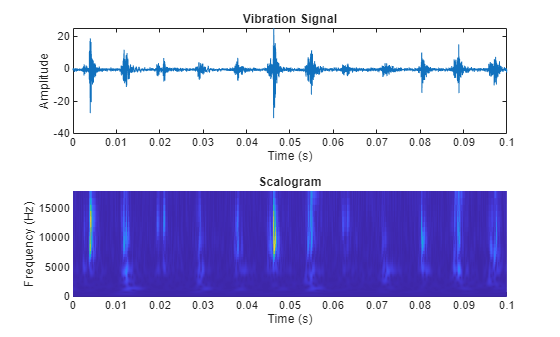
During the 0.1 seconds shown in the plot, the vibration signal contains 12 impulses because the tested bearing's BPFI is 118.875 Hz. Accordingly, the scalogram shows 12 distinct peaks that align with the impulses in the vibration signal.
The number of distinct peaks is a good feature to differentiate between inner race faults, outer race faults, and normal conditions. Therefore, a scalogram can be a good candidate for classifying bearing faults. In this example, all bearing signal measurements come from tests using the same shaft speed. To apply this example to bearing signals under different shaft speeds, the data needs to be normalized by shaft speed. Otherwise, the number of "pillars" in the scalogram will be wrong.
Prepare Training Data
The downloaded dataset contains a training dataset with 14 MAT files (two normal, five inner race fault, seven outer race fault) and a testing dataset with six MAT files (one normal, two inner race fault, three outer race fault).
Create a signal datastore, specifying a custom read function. The custom read function, customRead, is defined at the end of this example and reads data from a MAT file and returns a table of data, including the type of fault and the vibration signal. It requires an input of "gpu"or "cpu" that determines whether the vibration signal is returned as a gpuArray or an in-memory array. Specify "gpu".
fileLocationTrain = fullfile(".","RollingElementBearingFaultDiagnosis-Data","train_data");
dsTrainGPU = signalDatastore(fileLocationTrain,ReadFcn=@(filename) customRead(filename,"gpu"));
Now, convert the 1-D vibration signals to scalograms and save the images for training. The size of each scalogram is 227-by-227-by-3, which is the same input size required by SqueezeNet. To improve training accuracy use the convertSignalToScalogram function to extract the envelope of the raw signal and divide it into multiple segments. The convertSignalToScalogram function is defined at the end of this example. As the vibration signal data is a gpuArray, the convertSignalToScalogram function performs most of its operations of the GPU. The function creates a folder named train_image in the current folder and saves all scalogram images of the bearing signals in the RollingElementBearingFaultDiagnosis-Data/train_data folder to the train_image folder.
folderNameTrain = "train_image";
writeFiles = true;
convertSignalsToScalogram(dsTrainGPU,folderNameTrain,writeFiles);
Create an image datastore and split the training data into training and validation data sets, using 80% of the images from the train_image folder for training and 20% for validation.
path = fullfile(".",folderNameTrain);
imds = imageDatastore(path,IncludeSubfolders=true,LabelSource="foldernames");

[imdsTrain,imdsValidation] = splitEachLabel(imds,0.8,"randomize");
Train Network with Transfer Learning
Transfer learning is commonly used in deep learning applications. You can take a pretrained network and use it as a starting point for a new task. Using transfer learning is usually much faster and easier than training a network from scratch. You can quickly transfer learned features using a smaller number of training images.
Load a pretrained SqueezeNet neural network into the workspace by using the imagePretrainedNetwork function. To return a neural network ready for retraining for the new data, specify the number of classes. When you specify the number of classes, the imagePretrainedNetwork function adapts the neural network so that it outputs prediction scores for each of the specified number of classes.
numClasses = numel(categories(imdsTrain.Labels));
net = imagePretrainedNetwork("squeezenet",NumClasses=numClasses);
SqueezeNet uses the final convolutional layer conv10 to extract image features and classify the input image. This layer contains information to combine the features that the network extracts into class probabilities, a loss value, and predicted labels. To retrain the network for classifying new images, increase the learn rate of the weights and biases of the convolutional layer conv10.
net = setLearnRateFactor(net,"conv10","Weights",10);
net = setLearnRateFactor(net,"conv10","Bias",10);
Specify the training options:
To slow down learning, set the initial learning rate to a small value. The learning rate for each layer is the global learning rate multiplied by the learning rate of that layer. Therefore, increasing the learning rate for the last convolutional layer and specifying a low initial learning rate using the
trainingOptionsfunction results in fast learning only in the last convolutional layer and slower learning in the other layers.Train for four epochs. When performing transfer learning, you do not need to train for as many epochs. An epoch is a full training cycle on the entire training data set.
Use a mini-batch size of 20.
Shuffle the data every epoch.
Specify the validation data and validation frequency. The software validates the network every
ValidationFrequencyiterations during training.Display the training progress and disable the verbose output.
numEpochs = 4;
options = trainingOptions("sgdm", ...
  InitialLearnRate=0.0001, ...
  MaxEpochs=numEpochs, ...
  MiniBatchSize=20, ...
  Shuffle="every-epoch", ...
  ValidationData=imdsValidation, ...
  ValidationFrequency=30, ...
  Verbose=false, ...
  Plots="training-progress");
Train the new network and set the loss function to "crossentropy" (for classification problems). By default, trainnet uses a GPU if you have Parallel Computing Toolbox™ and a supported GPU device. Otherwise, trainnet uses a CPU. You can also specify the execution environment by using the ExecutionEnvironment name-value argument of trainingOptions.
trainedNet = trainnet(imdsTrain,net,"crossentropy",options);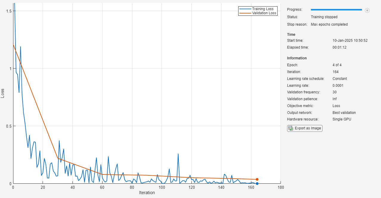
Validate Using Test Data Sets
Use bearing signals in the RollingElementBearingFaultDiagnosis-Data/test_data folder to validate the accuracy of the trained network. The test data needs to be processed in the same way as the training data.
Create a signal datastore to extract the vibration signals and store them in a test folder.
fileLocationTest = fullfile(".","RollingElementBearingFaultDiagnosis-Data","test_data");
dsTest = signalDatastore(fileLocationTest,ReadFcn=@(filename) customRead(filename,"gpu"));
Extract the labels using the filenames2labels function.
labels = filenames2labels(dsTest,ExtractBefore="_");Convert 1-D signals to 2-D scalograms using the covertToScalogram function.
folderNameTest = "test_image";
writeFiles = true;
convertSignalsToScalogram(dsTest,folderNameTest,writeFiles);
Create an image datastore to store the test images.
path = fullfile(".","test_image");
imdsTest = imageDatastore(path,IncludeSubfolders=true,LabelSource="foldernames");
Classify the test image datastore with the trained network. By default, the minibatchpredict function uses a GPU if one is available.
scores = minibatchpredict(trainedNet,imdsTest,MiniBatchSize=20);
YPred = scores2label(scores,unique(imdsTrain.Labels));
Compute the accuracy of the prediction.
YTest = imdsTest.Labels;
accuracy = sum(YPred == YTest)/numel(YTest)
accuracy =
0.9893
Plot a confusion matrix.
figure
confusionchart(YTest,YPred)
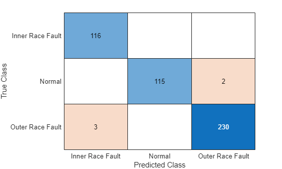
When you train the network multiple times, you might see some variation in accuracy between trainings, but the average accuracy should be around 98%. Even though the training set is quite small, this example benefits from transfer learning and achieves good accuracy.
Time Execution of Data Preprocessing and Training
Time the execution of the convertSignalsToScalogram function on the GPU. To time function execution on the GPU more accurately, use the wait function to block execution in MATLAB until the GPU completes its calculations.
tic
convertSignalsToScalogram(dsTrainGPU,folderNameTrain,writeFiles);
wait(gpu);
tExtractWithWriteGPU = toc
tExtractWithWriteGPU =
23.0715
For comparison, time the same function running on the CPU.
dsTrainCPU = signalDatastore(fileLocationTrain,ReadFcn=@(filename) customRead(filename,"cpu"));

tic
convertSignalsToScalogram(dsTrainCPU,folderNameTrain,writeFiles);
tExtractWithWriteCPU = toc
tExtractWithWriteCPU = 48.4499
The convertSignalsToScalogram function spends significant time writing the scalogram images to file. Time the execution of just reading from the datastore and creating the scalogram images on the CPU and the GPU by setting the writeFiles option to false.
writeFiles = false;
tic
convertSignalsToScalogram(dsTrainGPU,folderNameTrain,writeFiles);
wait(gpu);
tOnlyExtractGPU = toc
tOnlyExtractGPU =
16.7610
tic
convertSignalsToScalogram(dsTrainCPU,folderNameTrain,writeFiles);
tOnlyExtractCPU = toc
tOnlyExtractCPU =
39.1283
Time training the network on the GPU and CPU. To train the network on the CPU, set the ExecutionEnvironment training option to "cpu". Divide the total training time by the number of epochs to determine the per-epoch training time.
options.Plots = "none";
tic
trainedNet = trainnet(imdsTrain,net,"crossentropy",options);
wait(gpu);
tTrainGPUPerEpoch = toc/numEpochs
tTrainGPUPerEpoch =
3.7739
options.ExecutionEnvironment = "cpu";
tic
trainedNet = trainnet(imdsTrain,net,"crossentropy",options);
tTrainCPUPerEpoch = toc/numEpochs
tTrainCPUPerEpoch =
38.7324
Compare the execution times.
figure
b = bar([tExtractWithWriteCPU tExtractWithWriteGPU; ...
    tOnlyExtractCPU tOnlyExtractGPU; ...
    tTrainCPUPerEpoch tTrainGPUPerEpoch],"grouped");
b(1).Labels = round(b(1).YData,1);
b(2).Labels = round(b(2).YData,1);
xticklabels(["Data extraction and write" "Data extraction only" "Training"])
ylabel("Execution Time (s)")
legend(["CPU execution" "GPU execution"],Location="northeastoutside")

fprintf("Data extraction and write speedup: %3.1fx\nData extraction speedup: %3.1fx\nTraining speedup: %3.1fx", ...
    tExtractWithWriteCPU/tExtractWithWriteGPU,tOnlyExtractCPU/tOnlyExtractGPU,tTrainCPUPerEpoch/tTrainGPUPerEpoch);
Data extraction and write speedup: 2.1x
Data extraction speedup: 2.3x
Training speedup: 10.3x
Conclusion
Processing the data and training the network is significantly faster on the GPU.
Running your code on a GPU is straightforward and can provide a significant speedup for many workflows. Generally, using a GPU is more beneficial when you are performing computations on larger amounts of data, though the speedup you can achieve depends on your specific hardware and code.
References
[1] Randall, Robert B., and Jérôme Antoni. “Rolling Element Bearing Diagnostics—A Tutorial.” Mechanical Systems and Signal Processing 25, no. 2 (February 2011): 485–520. https://doi.org/10.1016/j.ymssp.2010.07.017.
[2] Bechhoefer, Eric. "Condition Based Maintenance Fault Database for Testing Diagnostics and Prognostic Algorithms.
[3] Verstraete, David, Andrés Ferrada, Enrique López Droguett, Viviana Meruane, and Mohammad Modarres. “Deep Learning Enabled Fault Diagnosis Using Time-Frequency Image Analysis of Rolling Element Bearings.” Shock and Vibration 2017 (2017): 1–17. https://doi.org/10.1155/2017/5067651.
Helper Functions
The plotBearingSignalAndScalogram function converts 1-D vibration signals in the MFPT dataset to 2-D scalograms. The function plots a vibration signal and its scalogram.
function plotBearingSignalAndScalogram(data)

fs = data.bearing.sr;
t_total = 0.1; % seconds
n = round(t_total*fs);
bearing = data.bearing.gs(1:n);
[cfs,frq] = cwt(bearing,"amor",fs);

% Plot the original signal and its scalogram
figure
tiledlayout(2,1)
nexttile
plot(0:1/fs:(n-1)/fs,bearing)
xlim([0 0.1])
title("Vibration Signal")
xlabel("Time (s)")
ylabel("Amplitude")

nexttile
surface(0:1/fs:(n-1)/fs,frq,abs(cfs))
shading flat
xlim([0 0.1])
ylim([0 max(frq)])
title("Scalogram")
xlabel("Time (s)")
ylabel("Frequency (Hz)")

end
The customRead function reads data from a MAT file and returns a table of data, including the type of fault and the vibration signal. It requires an input of "gpu"or "cpu" that determines whether the vibration signal is returned as a gpuArray or an in-memory array.
function data = customRead(filename,env)

mfile = matfile(filename); % Allows partial loading
[~,fname] = fileparts(filename);
bearing = mfile.bearing;

% Get label from filename.
cfname = char(fname);
switch cfname(1:3)
    case 'bas'
        label = "Normal";
    case 'Inn'
        label = "Inner Race Fault";
    case 'Out'
        label = "Outer Race Fault";
    otherwise
        label = "Unknown";
end
if env=="gpu"
    gs = gpuArray(bearing.gs);
else
    gs = bearing.gs;
end
data = table({gs},bearing.sr,mfile.BPFO,mfile.BPFI,label,string(fname), ...
    VariableNames=["gs" "sr" "BPFO" "BPFI" "Label" "FileName"]);
end
The convertSignalsToScalogram function extracts the envelope of the raw vibration signals in datastore ds and divides them into multiple segments. If writeFiles is true, the function creates a folder named folderName in the current folder and writes the scalogram images to the new folder.
function convertSignalsToScalogram(ds,folderName,writeFiles)
reset(ds)
while hasdata(ds)
    % Convert 1-D signals to scalograms and save scalograms as images
    data = read(ds);
    fs = data.sr;
    x = data.gs{:};
    label = data.Label;
    ratio = 5000/97656;
    interval = ratio*fs;
    N = floor(numel(x)/interval);

    if writeFiles
        % Create folder to save images
        fname = string(data.FileName);
        path = fullfile(".",folderName,label);
        if ~exist(path,"dir")
            mkdir(path);
        end
    end

    x = framesig(x,interval,OverlapLength=0);
    sig = envelope(x);
    for idx = 1:N
        cfs = cwt(sig(:,idx),"amor",seconds(1/fs));
        cfs = abs(cfs);
        img = ind2rgb(round(rescale(flip(cfs),0,255)),jet(320));
        img = imresize(img,[227 227]);
        if writeFiles
            outfname = fullfile(".",path,fname+"-"+num2str(idx)+".jpg");
            imwrite(img,outfname);
        end
    end
end
end
See Also
gpuArray (Parallel Computing Toolbox) | trainingOptions (Deep Learning Toolbox) | trainnet (Deep Learning Toolbox) | imagePretrainedNetwork (Deep Learning Toolbox) | analyzeNetwork (Deep Learning Toolbox) | convolution2dLayer (Deep Learning Toolbox) | confusionchart (Deep Learning Toolbox)