Train Discrete Soft Actor Critic Agent for Lander Vehicle

This example shows how to train a discrete soft actor critic (DSAC) agent with a discrete action space to land an airborne vehicle on the ground. For more information on DSAC agents, see Soft Actor-Critic (SAC) Agent.

Overview

The soft actor critic (SAC) is a stochastic off-policy reinforcement learning algorithm [1] and [2]. Since SAC is an off-policy algorithm, it can learn from the data stored over the episodes, which results in better sample efficiency and robustness. In this example, you train a SAC agent with discrete action space to solve a challenging lander environment. For more details on the lander environment, see Train PPO Agent for a Lander Vehicle.

Fix Random Seed Generator for Reproducibility

The example code may involve computation of random numbers at various stages such as initialization of the agent, creation of the actor and critic, resetting the environment during simulations, generating observations (for stochastic environments), generating exploration actions, and sampling min-batches of experiences for learning. Fixing the random number stream preserves the sequence of the random numbers every time you run the code and improves the likelihood to reproduce the results. You will fix the random number stream at various locations in the example. Fix the random number stream with a seed 0, using the Mersenne Twister random number algorithm. For more information on random number generation, see rng.

previousRngState = rng(0,"twister")

previousRngState = struct with fields:
     Type: 'twister'
     Seed: 0
    State: [625x1 uint32]

The output previousRngState is a structure that contains information about the previous state of the stream. You will restore the state at the end of the example.

Create Environment Object

Create the environment object using the LanderVehicle class provided in the example folder.

env = LanderVehicle

env = 
  LanderVehicle with properties:

                Mass: 1
                  L1: 10
                  L2: 5
             Gravity: 9.8060
        ThrustLimits: [0 8.5000]
                  Ts: 0.1000
               State: [6x1 double]
          LastAction: [2x1 double]
         LastShaping: 0
    DistanceIntegral: 0
    VelocityIntegral: 0
           TimeCount: 0

Get the observation and action specifications for the environment.

obsInfo = getObservationInfo(env);
actInfo = getActionInfo(env);

Create Discrete SAC Agent

Fix the random stream for reproducibility.

rng(0,"twister");

Discrete SAC agents use one or two vector Q-value function critics. This example uses two critics to mitigate overestimation in the critic target.

A discrete vector Q-value function takes only the observation as input and returns as output a single vector with as many elements as the number of possible discrete actions. The value of each output element represents the expected discounted cumulative long-term reward for taking the action corresponding to the element number, from the state corresponding to the current observation, and following the policy afterwards.

To model the parametrized vector Q-value function within the critics, use a neural network with one input layer (receiving the content of the observation channel, as specified by obsInfo) and one output layer (returning the vector of values for all the possible actions, as specified by actInfo).

Define the network for the critics as an array of layer objects. Note that numel(actInfo.Elements) returns the number of elements of the discrete action space.

hiddenLayerSize_Critic = [400, 300];
criticNetLayers = [  
    featureInputLayer(obsInfo.Dimension(1))
    fullyConnectedLayer(hiddenLayerSize_Critic(1))
    reluLayer
    fullyConnectedLayer(hiddenLayerSize_Critic(2))
    reluLayer
    fullyConnectedLayer(numel(actInfo.Elements)) 
    ];

Create the dlnetwork object criticNet1 and display the number of weights.

criticNet1 = dlnetwork(criticNetLayers);
summary(criticNet1)

   Initialized: true

   Number of learnables: 126.2k

   Inputs:
      1   'input'   7 features

Create the first critic approximator object using criticNet1, the observation specification and the action specification. For more information on Q-value function approximator, see rlVectorQValueFunction.

critic1 = rlVectorQValueFunction(criticNet1,obsInfo,actInfo);

Create the dlnetwork object criticNet2.

criticNet2 = dlnetwork(criticNetLayers);

Create the second critic approximator object using criticNet2, the observation specification and the action specification.

critic2 = rlVectorQValueFunction(criticNet2,obsInfo,actInfo);

The discrete SAC agents use a parameterized stochastic policy, which for discrete action spaces is implemented by a discrete categorical actor. This actor takes an observation as input and returns as output a random action sampled (among the finite number of possible actions) from a categorical probability distribution.

To model the parameterized policy within the actor, use a neural network with one input layer (which receives the content of the environment observation channel, as specified by obsInfo) and one output layer. The output layer must return a vector of probabilities for each possible actions, as specified by actInfo.

Define the network as an array of layer objects.

hiddenLayerSize_Actor = [400, 300];
actorNetLayers = [  
    featureInputLayer(obsInfo.Dimension(1))
    fullyConnectedLayer(hiddenLayerSize_Actor(1))
    reluLayer
    fullyConnectedLayer(hiddenLayerSize_Actor(2))
    reluLayer
    fullyConnectedLayer(numel(actInfo.Elements))
    ];

Convert the array of layers to a dlnetwork object and display the number of weights.

actorNet = dlnetwork(actorNetLayers);
summary(actorNet)

   Initialized: true

   Number of learnables: 126.2k

   Inputs:
      1   'input'   7 features

Create the actor using actorNet and the observation and action specifications. For more information on discrete categorical actors, see rlDiscreteCategoricalActor.

actor = rlDiscreteCategoricalActor(actorNet,obsInfo,actInfo);

Update the actor and critic neural networks using the Adam algorithm with a learning rate of 1e-3 and gradient threshold of 1. To create optimizer options for the actor and critic, use rlOptimizerOptions.

criticOptions = rlOptimizerOptions(...
    Optimizer="adam", ...
    LearnRate=1e-3, ... 
    GradientThreshold=1, ...
    L2RegularizationFactor=2e-4);

actorOptions = rlOptimizerOptions(...
    Optimizer="adam", ...
    LearnRate=1e-3, ...
    GradientThreshold=1, ...
    L2RegularizationFactor=1e-5);

Use a buffer of size 1e6 to store experiences, and a mini-batch of size 300 to update the critics and actor networks. The discount factor and target smoothing factor are to 0.99 and 1e-3, respectively. For a list of available DSAC agent hyperparameters, see rlSACAgentOptions.

Set the agent options.

agentOptions = rlSACAgentOptions;
agentOptions.SampleTime = env.Ts;
agentOptions.DiscountFactor = 0.99;
agentOptions.TargetSmoothFactor = 1e-3;
agentOptions.ExperienceBufferLength = 1e6;
agentOptions.MiniBatchSize = 300;
agentOptions.EntropyWeightOptions.EntropyWeight = 0.05;
agentOptions.EntropyWeightOptions.TargetEntropy = 0.5;

Set optimizer options for the actor and critic.

agentOptions.CriticOptimizerOptions = criticOptions;
agentOptions.ActorOptimizerOptions = actorOptions;

Create the discrete SAC agent.

agent = rlSACAgent(actor,[critic1 critic2],agentOptions);

Train Agent

Fix the random stream for reproducibility.

rng(0,"twister");

Create the evaluator object to run 5 evaluation episodes every 20 training episodes. For more information, see rlEvaluator.

evl = rlEvaluator(EvaluationFrequency=20, NumEpisodes=5);

To train the agent, first specify the training options using rlTrainingOptions. For this example, use the following options:

• Run each training for at most 5000 episodes, with each episode lasting at most 600 time steps.

• To speed up training, set the UseParallel option to true, which requires Parallel Computing Toolbox™ software. If you do not have the software installed set the option to false.

• Stop the training when the the average cumulative reward over the evaluation episodes reaches 450.

trainOpts = rlTrainingOptions;
trainOpts.Plots = 'training-progress';
trainOpts.MaxEpisodes = 10000;
trainOpts.MaxStepsPerEpisode = 600;
trainOpts.Verbose = 1;
trainOpts.StopTrainingCriteria = 'EvaluationStatistic';
trainOpts.StopTrainingValue = 450;
trainOpts.UseParallel = true;
trainOpts.ScoreAveragingWindowLength = 100;

Train the agent. Due to the complexity of the environment, the training process is computationally intensive and takes several hours to complete. To save time while running this example, load a pretrained agent by setting doTraining to false. For more information on training agents, see train and Train Reinforcement Learning Agents.

doTraining = false;
if doTraining   
    trainingStats = train(agent, env, trainOpts,Evaluator=evl);
else
    load("landerVehicleDSACAgent.mat");
end

An example training session is shown below. Your results can differ because of randomness in the training process.

Simulate Trained Agent

Set the random seed for simulation reproducibility.

rng(0,"twister");

Plot the environment first to create a visualization for the lander vehicle.

plot(env)

Set up simulation options to perform 5 simulations and set UseExplorationPolicy to false to use the trained greedy policy without exploration. For more information, see rlSimulationOptions.

simOptions = rlSimulationOptions(MaxSteps=600);
simOptions.NumSimulations = 10;

Do not use exploration in simulation.

agent.UseExplorationPolicy = false;

Simulate the trained agent within the environment. For more information, see sim.

experience = sim(env,agent,simOptions);

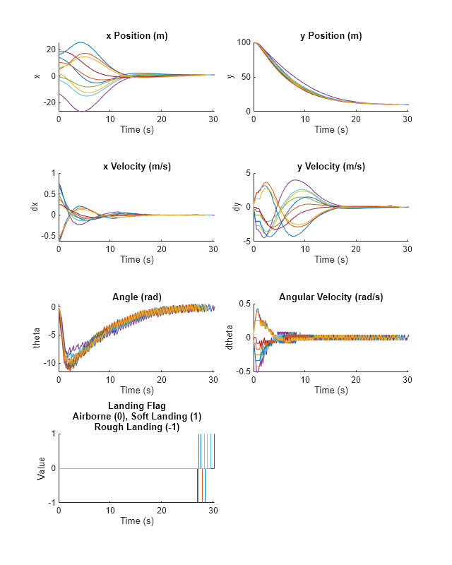
Plot the time history of the states for all simulations using the helper function plotLanderVehicleTrajectory, provided in the example folder.

% Observations to plot
obsToPlot = ["x","y","dx","dy","theta","dtheta","landing"];

% Create a figure
f = figure();
f.Position(3:4) = [800,1000];

% Create a tiled layout for the plots
t = tiledlayout(f,4,2,TileSpacing="compact");

% Plot the data
for ct = 1:numel(obsToPlot)
    ax = nexttile(t);
    plotLanderVehicleTrajectory(ax,experience,env,obsToPlot(ct));
end

Restore the random number stream using the information stored in previousRngState.

rng(previousRngState);

References

[1] Haarnoja, Tuomas, Aurick Zhou, Kristian Hartikainen, George Tucker, Sehoon Ha, Jie Tan, Vikash Kumar, et al. "Soft Actor-Critic Algorithms and Application." Preprint, submitted January 29, 2019. https://arxiv.org/abs/1812.05905.

[2] Christodoulou, Petros. “Soft Actor-Critic for Discrete Action Settings.” Preprint, submitted October 18, 2019. https://arxiv.org/abs/1910.07207.