Contenuto principale

cpsd

Cross power spectral density

Description

pxy = cpsd(x,y) estimates the Cross Power Spectral Density (CPSD) of two discrete-time signals, x and y, using Welch’s averaged, modified periodogram method of spectral estimation.

  • If x and y are both vectors, they must have the same length.

  • If one of the signals is a matrix and the other is a vector, then the length of the vector must equal the number of rows in the matrix. The function expands the vector and returns a matrix of column-by-column CPSD estimates.

  • If x and y are matrices with the same number of rows but different numbers of columns, then cpsd returns a three-dimensional array, pxy, containing CPSD estimates for all combinations of input columns. Each column of pxy corresponds to a column of x, and each page corresponds to a column of y: pxy(:,m,n) = cpsd(x(:,m),y(:,n)).

  • If x and y are matrices of equal size, then cpsd operates column-wise: pxy(:,n) = cpsd(x(:,n),y(:,n)). To obtain a multi-input/multi-output array, append "mimo" to the argument list.

The function returns either a one-sided or two-sided CPSD estimate if you specify x and y as real-valued or complex-valued signals, respectively.

example

pxy = cpsd(x,y,window) uses window to divide x and y into segments and perform windowing.

pxy = cpsd(x,y,window,nOverlap) uses nOverlap samples of overlap between adjoining segments.

pxy = cpsd(x,y,window,nOverlap,nfft) uses nfft sampling points to calculate the discrete Fourier transform.

pxy = cpsd(___,"mimo") computes a multi-input/multi-output array of CPSD estimates. This syntax can include any combination of input arguments from previous syntaxes.

example

[pxy,w] = cpsd(___) returns a vector of normalized frequencies, w, at which the function estimates the CPSD.

[pxy,f] = cpsd(___,Fs) returns a vector of frequencies, f, expressed in terms of the sample rate, Fs, at which the function estimates the CPSD. Fs must be the sixth numeric input to cpsd. To input a sample rate and still use the default values of the preceding optional arguments, specify these arguments as empty, [].

[pxy,w] = cpsd(x,y,window,nOverlap,w) returns the CPSD estimates at the normalized frequencies specified in w.

example

[pxy,f] = cpsd(x,y,window,nOverlap,f,Fs) returns the CPSD estimates at the frequencies specified in f.

example

[___] = cpsd(x,y,___,freqRange) returns the CPSD estimate over the frequency range specified by freqRange. Valid options for freqRange are "onesided", "twosided", and "centered".

[___] = cpsd(___,Parent=h) plots the CPSD estimate in the target parent container h. (since R2026a)

example

cpsd(___) with no output arguments plots the CPSD estimate in the current figure window.

example

Examples

collapse all

Generate two colored noise signals and plot their cross power spectral density. Specify a length-1024 FFT and a 500-point triangular window with 50% overlap between segments. Reset the random number generator for reproducible results.

rng("default")
r = randn(2e4,1);

hx = fir1(30,0.2,rectwin(31));
x = filter(hx,1,r);

hy = ones(1,10);
y = filter(hy,1,r);

win = triang(500);
nov = 250;

cpsd(x,y,win,nov,1024)

Figure contains an axes object. The axes object with title Welch Cross Power Spectral Density Estimate, xlabel Normalized Frequency ( times pi rad/sample), ylabel Power/Frequency (dB/(rad/sample)) contains an object of type line.

Generate two two-channel sinusoids sampled at 1 kHz for 1 second. The channels of the first signal have frequencies of 200 Hz and 300 Hz. The channels of the second signal have frequencies of 300 Hz and 400 Hz. Both signals are embedded in unit-variance white Gaussian noise. Reset the random number generator for reproducible results.

rng("default")
fs = 1e3;
t = (0:1/fs:1-1/fs)';

q = 2*sin(2*pi*[200 300].*t);
q = q + randn(size(q));

r = 2*sin(2*pi*[300 400].*t);
r = r + randn(size(r));

Compute the cross power spectral density of the two signals. Use a 256-sample Bartlett window to divide the signals into segments and window the segments. Specify 128 samples of overlap between adjoining segments and 2048 DFT points. Use the built-in functionality of cpsd to plot the result.

cpsd(q,r,bartlett(256),128,2048,fs)

Figure contains an axes object. The axes object with title Welch Cross Power Spectral Density Estimate, xlabel Frequency (Hz), ylabel Power/Frequency (dB/Hz) contains 2 objects of type line.

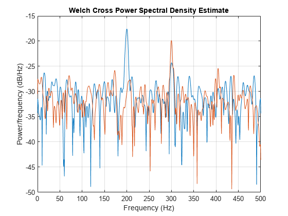
By default, cpsd works column-by-column on matrix inputs of the same size. Each channel peaks at the frequencies of the original sinusoids.

Repeat the calculation, but now append "mimo" to the list of arguments.

cpsd(q,r,bartlett(256),128,2048,fs,"mimo")

Figure contains an axes object. The axes object with title Welch Cross Power Spectral Density Estimate, xlabel Frequency (Hz), ylabel Power/Frequency (dB/Hz) contains 4 objects of type line.

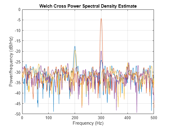
When called with the "mimo" option, cpsd returns a three-dimensional array containing cross power spectral density estimates for all combinations of input columns. The estimate of the second channel of q and the first channel of r shows an enhanced peak at the common frequency of 300 Hz.

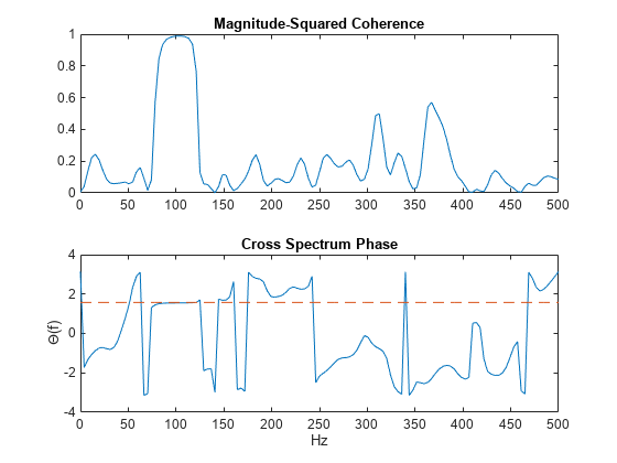
Generate two 100 Hz sinusoidal signals sampled at 1 kHz for 296 ms. One of the sinusoids lags the other by 2.5 ms, equivalent to a phase lag of π/2. Both signals are embedded in white Gaussian noise of variance 1/4². Reset the random number generator for reproducible results.

rng("default")
Fs = 1000;
t = 0:1/Fs:0.296;

x = cos(2*pi*t*100) + 0.25*randn(size(t));
tau = 1/400;
y = cos(2*pi*100*(t-tau)) + 0.25*randn(size(t));

Compute and plot the magnitude of the cross power spectral density. Use the default settings for cpsd. The magnitude peaks at the frequency where there is significant coherence between the signals.

cpsd(x,y,[],[],[],Fs)

Figure contains an axes object. The axes object with title Welch Cross Power Spectral Density Estimate, xlabel Frequency (Hz), ylabel Power/Frequency (dB/Hz) contains an object of type line.

Plot magnitude-squared coherence function and the phase of the cross spectrum. The ordinate at the high-coherence frequency corresponds to the phase lag between the sinusoids.

[Cxy,F] = mscohere(x,y,[],[],[],Fs);

[Pxy,~] = cpsd(x,y,[],[],[],Fs);

figure
tiledlayout("flow")
nexttile
plot(F,Cxy)
title("Magnitude-Squared Coherence")
nexttile
plot(F,angle(Pxy),F,2*pi*100*tau*ones(size(F)),"--")
xlabel("Hz")
ylabel("\Theta(f)")
title("Cross Spectrum Phase")

Figure contains 2 axes objects. Axes object 1 with title Magnitude-Squared Coherence contains an object of type line. Axes object 2 with title Cross Spectrum Phase, xlabel Hz, ylabel \Theta(f) contains 2 objects of type line.

Generate two N-sample exponential sequences, xa=an and xb=bn, with n0. Specify a=0.8, b=0.9, and a small N to see finite-size effects.

N = 10;
n = 0:N-1;

a = 0.8;
b = 0.9;

xa = a.^n;
xb = b.^n;

Compute and plot the cross power spectral density of the sequences over the complete interval of normalized frequencies, [-π,π]. Specify a rectangular window of length N and no overlap between segments.

w = -pi:1/1000:pi;
wind = rectwin(N);
nove = 0;

[pxx,f] = cpsd(xa,xb,wind,nove,w);

The cross power spectrum of the two sequences has an analytic expression for large N:

R(ω)=11-ae-jω11-bejω.

Convert this expression to a cross power spectral density by dividing it by 2πN. Compare the results. The ripple in the cpsd result is a consequence of windowing.

nfac = 2*pi*N;

X = 1./(1-a*exp(-1j*w));
Y = 1./(1-b*exp( 1j*w));
R = X.*Y/nfac;

semilogy(f/pi,abs(pxx))
hold on
semilogy(w/pi,abs(R))
hold off
legend(["cpsd" "Analytic"])
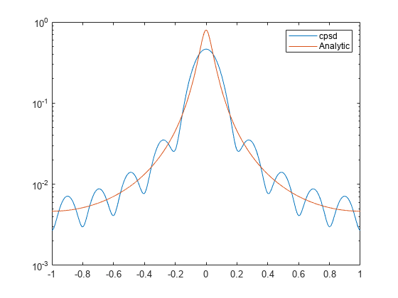
Figure contains an axes object. The axes object contains 2 objects of type line. These objects represent cpsd, Analytic.

Repeat the calculation with N=25. The curves agree to six figures for N as small as 100.

N = 25;
n = 0:N-1;
xa = a.^n;
xb = b.^n;

wind = rectwin(N);

[pxx,f] = cpsd(xa,xb,wind,nove,w);
R = X.*Y/(2*pi*N);

semilogy(f/pi,abs(pxx))
hold on
semilogy(w/pi,abs(R))
hold off
legend(["cpsd" "Analytic"])

Figure contains an axes object. The axes object contains 2 objects of type line. These objects represent cpsd, Analytic.

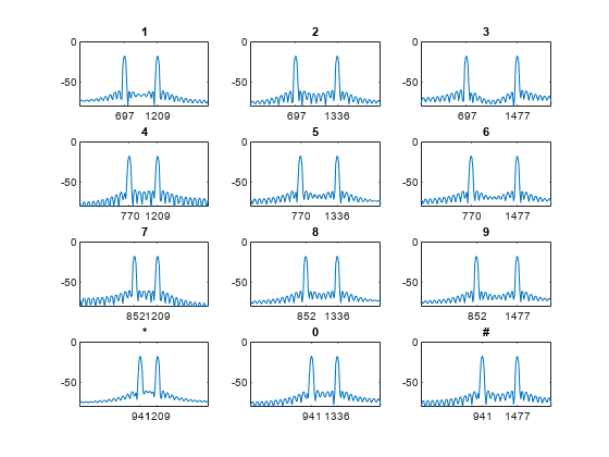
Use cross power spectral density to identify a highly corrupted tone.

The sound signals generated when you dial a number or symbol on a digital phone are sums of sinusoids with frequencies taken from two different groups. Each pair of tones contains one frequency of the low group (697 Hz, 770 Hz, 852 Hz, or 941 Hz) and one frequency of the high group (1209 Hz, 1336 Hz, or 1477 Hz).

Generate signals corresponding to all the symbols. Sample each tone at 4 kHz for half a second. Prepare a reference table.

fs = 4e3;
t = 0:1/fs:0.5-1/fs;

nms = ["1";"2";"3";"4";"5";"6";"7";"8";"9";"*";"0";"#"];

ver = [697 770 852 941];
hor = [1209 1336 1477];

v = length(ver);
h = length(hor);

for k = 1:v
    for l = 1:h
        idx = h*(k-1)+l;
        tone = sum(sin(2*pi*[ver(k);hor(l)].*t))';
        tones(:,idx) = tone;
    end
end

Plot the Welch periodogram of each signal and annotate the component frequencies. Use a 200-sample Hamming window to divide the signals into non-overlapping segments and window the segments.

[pxx,f] = pwelch(tones,hamming(200),0,[],fs);

for k = 1:v
    for l = 1:h
        idx = h*(k-1)+l;
        ax = subplot(v,h,idx);
        plot(f,pow2db(pxx(:,idx)))
        ylim([-80 0])
        title(nms(idx))
        tx = [ver(k);hor(l)];
        ax.XTick = tx;
        ax.XTickLabel = int2str(tx);
    end
end

Figure contains 12 axes objects. Axes object 1 with title 1 contains an object of type line. Axes object 2 with title 2 contains an object of type line. Axes object 3 with title 3 contains an object of type line. Axes object 4 with title 4 contains an object of type line. Axes object 5 with title 5 contains an object of type line. Axes object 6 with title 6 contains an object of type line. Axes object 7 with title 7 contains an object of type line. Axes object 8 with title 8 contains an object of type line. Axes object 9 with title 9 contains an object of type line. Axes object 10 with title * contains an object of type line. Axes object 11 with title 0 contains an object of type line. Axes object 12 with title # contains an object of type line.

A signal produced by dialing the number 8 is sent through a noisy channel. The received signal is so corrupted that the number cannot be identified by inspection. Reset the random number generator for reproducible results.

rng("default")
mys = sum(sin(2*pi*[ver(3);hor(2)].*t))' + 5*randn(size(t'));

% To hear, type soundsc(mys,fs)

Compute the cross power spectral density of the corrupted signal and the reference signals. Window the signals using a 512-sample Kaiser window with shape factor β = 5. Plot the magnitude of each spectrum.

[pxy,f] = cpsd(mys,tones,kaiser(512,5),100,[],fs);

for k = 1:v
    for l = 1:h
        idx = h*(k-1)+l;
        ax = subplot(v,h,idx);
        plot(f,pow2db(abs(pxy(:,idx))))
        ylim([-80 0])
        title(nms(idx))
        tx = [ver(k);hor(l)];
        ax.XTick = tx;
        ax.XTickLabel = int2str(tx);
    end
end

Figure contains 12 axes objects. Axes object 1 with title 1 contains an object of type line. Axes object 2 with title 2 contains an object of type line. Axes object 3 with title 3 contains an object of type line. Axes object 4 with title 4 contains an object of type line. Axes object 5 with title 5 contains an object of type line. Axes object 6 with title 6 contains an object of type line. Axes object 7 with title 7 contains an object of type line. Axes object 8 with title 8 contains an object of type line. Axes object 9 with title 9 contains an object of type line. Axes object 10 with title * contains an object of type line. Axes object 11 with title 0 contains an object of type line. Axes object 12 with title # contains an object of type line.

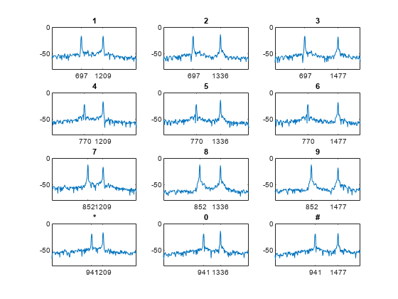
The digit in the corrupted signal has the spectrum with the highest peaks and the highest RMS value.

[~,loc] = max(rms(abs(pxy)));

digit = nms(loc)
digit = 
"8"

Since R2026a

Plot the Welch cross power spectral density (CPSD) estimate for a MIMO system in the specified target axes and panel containers.

Two masses connected to a spring and a damper on each side form an ideal one-dimensional discrete-time oscillating system. The system input array u consists of random driving forces applied to the masses. The system output array y contains the observed displacements of the masses from their initial reference positions. The system is sampled at a rate Fs of 40 Hz.

MIMO one-dimensional mass-spring-damper system. The damper and the spring form a parallel-connected section that connect to a wall or to a mass. From left to right: left wall, a damper-spring section, mass m1, a damper-spring section, a mass m2, a damper-spring section, right wall. m1=1 kilogram, m2=mu kilograms, the springs have elastic constants k Newton per meter, and the dampers have damping constant b kilograms per second. The displacements of the masses m1 and m2 are r1 and r2, respectively, in meters.

Load the data file containing the MIMO system inputs, the system outputs, and the sample rate. The example Frequency-Response Analysis of MIMO System analyzes the system that generated the data used in this example.

load MIMOdata Fs u y

Estimate the Welch CPSD of the system and plot the estimate on a UI axes. Divide the signal into 5000-sample segments with 50% overlap between adjoining segments. Apply a Hanning window to each segment and calculate the discrete Fourier transform of the signal segment using 1024 frequency points. Select the "mimo" option to produce all four estimates.

uif = uifigure(Position=[100 100 720 540]);
ax = uiaxes(uif,Position=[5 280 400 240]);

g = hann(5000);
ol = 2500;
nfft = 1024;

cpsd(u,y,g,ol,nfft,Fs,"mimo",Parent=ax)
legend(ax,"Input "+[1 2]+", Output "+[1 2]',Location="best")
title(ax,"Welch CPSD in UI Axes")

Figure contains an axes object. The axes object with title Welch CPSD in UI Axes, xlabel Frequency (Hz), ylabel Power/Frequency (dB/Hz) contains 4 objects of type line. These objects represent Input 1, Output 1, Input 1, Output 2, Input 2, Output 1, Input 2, Output 2.

Add a panel container in the southeastern corner of the UI figure window.

p = uipanel(uif,Position=[220 5 480 270], ...
    Title="Welch CPSD in Panel Container", ...
    BackgroundColor="white");

Plot the Welch CPSD estimate of each input-output pair of the system.

cpsd(u,y,g,ol,nfft,Fs,Parent=p)

Figure contains 2 axes objects and another object of type uipanel. Axes object 1 with title Welch Cross Power Spectral Density Estimate, xlabel Frequency (Hz), ylabel Power/Frequency (dB/Hz) contains 2 objects of type line. Axes object 2 with title Welch CPSD in UI Axes, xlabel Frequency (Hz), ylabel Power/Frequency (dB/Hz) contains 4 objects of type line. These objects represent Input 1, Output 1, Input 1, Output 2, Input 2, Output 1, Input 2, Output 2.

Input Arguments

collapse all

Input signals, specified as vectors or matrices.

Example: cos(pi/4*(0:159))+randn(1,160) specifies a sinusoid embedded in white Gaussian noise.

Data Types: single | double
Complex Number Support: Yes

Window, specified as an integer or as a row or column vector. Use window to divide the signal into segments.

  • If window is an integer, then cpsd divides x and y into segments of length window and windows each segment with a Hamming window of that length.

  • If window is a vector, then cpsd divides x and y into segments of the same length as the vector and windows each segment using window.

If the length of x and y cannot be divided exactly into an integer number of segments with nOverlap overlapping samples, then the signals are truncated accordingly.

If you specify window as empty, then cpsd uses a Hamming window such that x and y are divided into eight segments with nOverlap overlapping samples.

For a list of available windows, see Windows.

Example: hann(N+1) and (1-cos(2*pi*(0:N)'/N))/2 both specify a Hann window of length N + 1.

Data Types: single | double

Number of overlapped samples, specified as a positive integer.

  • If window is scalar, then nOverlap must be smaller than window.

  • If window is a vector, then nOverlap must be smaller than the length of window.

If you specify nOverlap as empty, then cpsd uses a number that produces 50% overlap between segments. If the segment length is unspecified, the function sets nOverlap to ⌊N/4.5⌋, where N is the length of the input and output signals.

Data Types: double | single

Number of DFT points, specified as a positive integer. If you specify nfft as empty, then cpsd sets the parameter to max(256,2p), where p = ⌈log2 N for input signals of length N.

Data Types: single | double

Sample rate, specified as a positive scalar. The sample rate is the number of samples per unit time. If the unit of time is seconds, then the sample rate is in Hz.

  • If you specify Fs as empty [], then cpsd assumes that the input signal x has a sample rate of 1 Hz.

  • If you do not specify Fs, then cpsd assumes that the input signal x has a sample rate of 2π rad/sample.

Normalized frequencies, specified as a row or column vector with at least two elements. Normalized frequencies are in rad/sample.

Example: w = [pi/4 pi/2]

Data Types: double | single

Frequencies, specified as a row or column vector with at least two elements. The frequencies are in cycles per unit time. The unit time is specified by the sample rate, fs. If fs has units of samples/second, then f has units of Hz.

Example: fs = 1000; f = [100 200]

Data Types: double | single

Frequency range for cross power spectral density (CPSD) estimate, specified as "onesided", "twosided", or "centered". The default is "onesided" for real-valued signals and "twosided" for complex-valued signals.

  • "onesided" — Returns the one-sided estimate of the CPSD of two real-valued input signals, x and y. If nfft is even, pxy has nfft/2 + 1 rows and is computed over the interval [0,π] rad/sample. If nfft is odd, pxy has (nfft + 1)/2 rows and the interval is [0,π) rad/sample. If you specify Fs, the corresponding intervals are [0,Fs/2] cycles/unit time for even nfft and [0,Fs/2) cycles/unit time for odd nfft.

  • "twosided" — Returns the two-sided estimate of the CPSD of two real-valued or complex-valued input signals, x and y. In this case, pxy has nfft rows and is computed over the interval [0,2π) rad/sample. If you specify Fs, the interval is [0,Fs) cycles/unit time.

  • "centered" — Returns the centered two-sided estimate of the CPSD of two real-valued or complex-valued input signals, x and y. In this case, pxy has nfft rows and is computed over the interval (–π,π] rad/sample for even nfft and (–π,π) rad/sample for odd nfft. If you specify Fs, the corresponding intervals are (–Fs/2, Fs/2] cycles/unit time for even nfft and (–Fs/2, Fs/2) cycles/unit time for odd nfft.

If you specify a vector w or f of frequencies and freqRange as inputs, then cpsd ignores freqRange.

Since R2026a

Target parent container, specified as an Axes object, a UIAxes object, or a Panel object.

If you specify Parent=h, the cpsd function plots the Welch CPSD estimate on the specified target parent container, whether you call the function with or without output arguments.

For more information about target containers and the parent-child relationship in MATLAB® graphics, see Graphics Object Hierarchy. For more information about using Parent in UIAxes and Panel objects to design apps, see Plot Spectral Representations of Signal in App Designer.

Example: h = axes(figure,Position=[0.1 0.1 0.6 0.5]) defines an axes parent container. When you specify cpsd(x,y,[],[],[],Parent=h), the function plots the Welch CPSD estimate of the signals x and y in the parent container h.

Output Arguments

collapse all

Cross power spectral density, returned as a vector, matrix, or three-dimensional array.

Normalized frequencies, returned as a real-valued column vector.

  • If pxy is one-sided, w spans the interval [0,π] when nfft is even and [0,π) when nfft is odd.

  • If pxy is two-sided, w spans the interval [0,2π).

  • If pxy is DC-centered, w spans the interval (–π,π] when nfft is even and (–π,π) when nfft is odd.

Data Types: double | single

Frequencies, returned as a real-valued column vector.

Data Types: double | single

More About

collapse all

Algorithms

cpsd uses Welch’s averaged, modified periodogram method of spectral estimation.

References

[1] Oppenheim, Alan V., Ronald W. Schafer, and John R. Buck. Discrete-Time Signal Processing. 2nd Ed. Upper Saddle River, NJ: Prentice Hall, 1999.

[2] Rabiner, Lawrence R., and B. Gold. Theory and Application of Digital Signal Processing. Englewood Cliffs, NJ: Prentice-Hall, 1975, pp. 414–419.

[3] Welch, Peter D. “The Use of the Fast Fourier Transform for the Estimation of Power Spectra: A Method Based on Time Averaging Over Short, Modified Periodograms.” IEEE® Transactions on Audio and Electroacoustics, Vol. AU-15, June 1967, pp. 70–73.

Extended Capabilities

expand all

C/C++ Code Generation
Generate C and C++ code using MATLAB® Coder™.

GPU Code Generation
Generate CUDA® code for NVIDIA® GPUs using GPU Coder™.

Version History

Introduced before R2006a

expand all