Main Content

modalfrf

Frequency-response functions for modal analysis

Description

example

frf = modalfrf(x,y,fs,window) estimates a matrix of frequency response functions, frf, from the excitation signals, x, and the response signals, y, all sampled at a rate fs. The output, frf, is an H1 estimate computed using Welch’s method with window to window the signals. x and y must have the same number of rows. If x or y is a matrix, each column represents a signal.

The system response, y, is assumed to contain acceleration measurements. To compute a frequency-response function starting from displacement or velocity measurements, use the 'Sensor' argument. modalfrf always outputs the frequency-response function in dynamic flexibility (receptance) format irrespective of the sensor type.

frf = modalfrf(x,y,fs,window,noverlap) specifies noverlap samples of overlap between adjoining segments.

example

frf = modalfrf(___,Name,Value) specifies options using name-value arguments, using any combination of inputs from previous syntaxes. Options include the estimator, the measurement configuration, and the type of sensor measuring the system response.

example

[frf,f,coh] = modalfrf(___) also returns the frequency vector corresponding to each frequency-response function, as well as the multiple coherence matrix.

[frf,f] = modalfrf(sys) computes the frequency-response function of the identified model sys. Use estimation commands like ssest (System Identification Toolbox), n4sid (System Identification Toolbox), or tfest (System Identification Toolbox) to create sys from time-domain input and output signals. This syntax allows use only of the 'Sensor' name-value argument. You must have a System Identification Toolbox™ license to use this syntax.

frf = modalfrf(sys,f) specifies the frequencies at which to compute frf. This syntax allows use only of the 'Sensor' name-value argument. You must have a System Identification Toolbox license to use this syntax.

example

modalfrf(___) with no output arguments plots the frequency response functions in the current figure. The plots are limited to the first four excitations and four responses.

Examples

collapse all

Visualize the frequency-response function of a single-input/single-output hammer excitation.

Load a data file that contains:

  • Xhammer An input excitation signal consisting of five hammer blows delivered periodically.

  • Yhammer The response of a system to the input. Yhammer is measured as a displacement.

The signals are sampled at 4 kHz. Plot the excitation and output signals.

load modaldata

subplot(2,1,1)
plot(thammer,Xhammer(:))
ylabel('Force (N)')
subplot(2,1,2)
plot(thammer,Yhammer(:))
ylabel('Displacement (m)')
xlabel('Time (s)')

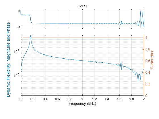
Compute and display the frequency-response function. Window the signals using a rectangular window. Specify that the window covers the period between hammer blows.

clf
winlen = size(Xhammer,1);
modalfrf(Xhammer(:),Yhammer(:),fs,winlen,'Sensor','dis')

Compute the frequency-response functions for a two-input/two-output system excited by random noise.

Load a data file that contains Xrand, the input excitation signal, and Yrand, the system response. Compute the frequency-response functions using a 5000-sample Hann window and 50% overlap between adjoining data segments. Specify that the output measurements are displacements.

load modaldata
winlen = 5000;

frf = modalfrf(Xrand,Yrand,fs,hann(winlen),0.5*winlen,'Sensor','dis');

Use the plotting functionality of modalfrf to visualize the responses.

modalfrf(Xrand,Yrand,fs,hann(winlen),0.5*winlen,'Sensor','dis')

Estimate the frequency-response function for a simple single-input/single-output system and compare it to the definition.

A one-dimensional discrete-time oscillating system consists of a unit mass, m, attached to a wall by a spring with elastic constant k=1. A sensor samples the displacement of the mass at Fs=1 Hz. A damper impedes the motion of the mass by exerting on it a force proportional to speed, with damping constant b=0.01.

Generate 3000 time samples. Define the sampling interval Δt=1/Fs.

Fs = 1;
dt = 1/Fs;
N = 3000;
t = dt*(0:N-1);
b = 0.01;

The system can be described by the state-space model

x(k+1)=Ax(k)+Bu(k),y(k)=Cx(k)+Du(k),

where x=[rv]T is the state vector, r and v are respectively the displacement and velocity of the mass, u is the driving force, and y=r is the measured output. The state-space matrices are

A=exp(AcΔt),B=Ac-1(A-I)Bc,C=[10],D=0,

I is the 2×2 identity, and the continuous-time state-space matrices are

Ac=[01-1-b],Bc=[01].

Ac = [0 1;-1 -b];
A = expm(Ac*dt);

Bc = [0;1];
B = Ac\(A-eye(2))*Bc;

C = [1 0];
D = 0;

The mass is driven by random input for the first 2000 seconds and then left to return to rest. Use the state-space model to compute the time evolution of the system starting from an all-zero initial state. Plot the displacement of the mass as a function of time.

rng default
u = randn(1,N)/2;
u(2001:end) = 0;

y = 0;
x = [0;0];
for k = 1:N
    y(k) = C*x + D*u(k);
    x = A*x + B*u(k);
end

plot(t,y)

Estimate the modal frequency-response function of the system. Use a Hann window half as long as the measured signals. Specify that the output is the displacement of the mass.

wind = hann(N/2);

[frf,f] = modalfrf(u',y',Fs,wind,'Sensor','dis');

The frequency-response function of a discrete-time system can be expressed as the Z-transform of the time-domain transfer function of the system, evaluated at the unit circle. Compare the modalfrf estimate with the definition.

[b,a] = ss2tf(A,B,C,D);

nfs = 2048;
fz = 0:1/nfs:1/2-1/nfs;
z = exp(2j*pi*fz);
ztf = polyval(b,z)./polyval(a,z);

plot(f,20*log10(abs(frf)))
hold on
plot(fz*Fs,20*log10(abs(ztf)))
hold off
grid
ylim([-60 40])

Estimate the natural frequency and the damping ratio for the vibration mode.

[fn,dr] = modalfit(frf,f,Fs,1,'FitMethod','PP')
fn = 0.1593
dr = 0.0043

Compare the natural frequency to 1/2π, which is the theoretical value for the undamped system.

theo = 1/(2*pi)
theo = 0.1592

Estimate the frequency-response function of a multi-input/multi-output (MIMO) system.

Two masses connected to a spring and a damper on each side form an ideal one-dimensional discrete-time oscillating system. The system input array u consists of random driving forces applied to the masses. The system output array y contains the observed displacements of the masses from their initial reference positions. The system is sampled at a rate Fs of 40 Hz.

Load the data file containing the MIMO system inputs, the system outputs, and the sample rate. The example Frequency-Response Analysis of MIMO System analyzes the system that generated the data used in this example.

load MIMOdata

Estimate and plot the modal frequency response functions of the system. Use a 12000-sample Hann window with 9000 samples of overlap between adjoining segments. Specify the sensor data type as measured displacements.

wind = hann(12000);
nove = 9000;

[frf,f] = modalfrf(u,y,Fs,wind,nove,Sensor="dis");

tiledlayout flow
for jk = 1:2
    for kj = 1:2
        nexttile
        plot(f,mag2db(abs(frf(:,jk,kj))))
        grid on
        axis([0 Fs/2 -100 0])
        title("Input "+jk+", Output "+kj)
        xlabel("Frequency (Hz)")
        ylabel("Magnitude (dB)")
    end
end

Compute the frequency-response function of a two-input/six-output data set corresponding to a steel frame.

Load a structure containing the input excitations and the output accelerometer measurements. The system is sampled at 1024 Hz for about 3.9 seconds.

load modaldata SteelFrame
X = SteelFrame.Input;
Y = SteelFrame.Output;
fs = SteelFrame.Fs;

Use the subspace method to compute the frequency-response functions. Divide the input and output signals into nonoverlapping, 1000-sample segments. Window each segment using a rectangular window. Specify a model order of 36.

[frf,f] = modalfrf(X,Y,fs,1000,'Estimator','subspace','Order',36);

Visualize the stabilization diagram for the system. Identify up to 15 physical modes.

modalsd(frf,f,fs,'MaxModes',15)

Input Arguments

collapse all

Excitation signals, specified as a vector or matrix.

Data Types: single | double

Response signals, specified as a vector or matrix.

Data Types: single | double

Sample rate, specified as a positive scalar expressed in hertz.

Data Types: single | double

Window, specified as an integer or as a row or column vector. Use window to divide the signal into segments:

  • If window is an integer, then modalfrf divides x and y into segments of length window and windows each segment with a rectangular window of that length.

  • If window is a vector, then modalfrf divides x and y into segments of the same length as the vector and windows each segment using window.

  • If 'Estimator' is specified as 'subspace', then modalfrf ignores the shape of window and uses its length to determine the number of frequency points in the returned frequency-response function.

If the length of x and y cannot be divided exactly into an integer number of segments with noverlap overlapping samples, then the signals are truncated accordingly.

For a list of available windows, see Windows.

Example: hann(N+1) and (1-cos(2*pi*(0:N)'/N))/2 both specify a Hann window of length N + 1.

Data Types: single | double

Number of overlapped samples, specified as a positive integer.

  • If window is a scalar, then noverlap must be smaller than window.

  • If window is a vector, then noverlap must be smaller than the length of window.

Data Types: double | single

Identified system, specified as a model with identified parameters. Use estimation commands like ssest (System Identification Toolbox), n4sid (System Identification Toolbox), or tfest (System Identification Toolbox) to create sys from time-domain input and output signals. See Modal Analysis of Identified Models for an example. Syntaxes that use sys typically require less data than syntaxes that use nonparametric methods. You must have a System Identification Toolbox license to use this input argument.

Example: idss([0.5418 0.8373;-0.8373 0.5334],[0.4852;0.8373],[1 0],0,[0;0],[0;0],1) generates an identified state-space model corresponding to a unit mass attached to a wall by a spring of unit elastic constant and a damper with constant 0.01. The displacement of the mass is sampled at 1 Hz.

Example: idtf([0 0.4582 0.4566],[1 -1.0752 0.99],1) generates an identified transfer-function model corresponding to a unit mass attached to a wall by a spring of unit elastic constant and a damper with constant 0.01. The displacement of the mass is sampled at 1 Hz.

Frequencies, specified as a vector expressed in Hz.

Data Types: single | double

Name-Value Arguments

Specify optional pairs of arguments as Name1=Value1,...,NameN=ValueN, where Name is the argument name and Value is the corresponding value. Name-value arguments must appear after other arguments, but the order of the pairs does not matter.

Before R2021a, use commas to separate each name and value, and enclose Name in quotes.

Example: 'Sensor','vel','Est','H1' specifies that the input signal consists of velocity measurements and that the estimator of choice is H1.

Estimator, specified as 'H1', 'H2', 'Hv', or 'subspace'. See Transfer Function for more information about the H1 and H2 estimators.

  • Use 'H1' when the noise is uncorrelated with the excitation signals.

  • Use 'H2' when the noise is uncorrelated with the response signals. In this case, the number of excitation signals must equal the number of response signals.

  • Use 'Hv' to minimize the discrepancy between modeled and estimated response data by minimizing the trace of the error matrix. Hv is the geometric mean of H1 and H2: Hv = (H1H2)1/2

    The measurement must be single-input/single-output (SISO).

  • Use 'subspace' to compute the frequency-response functions using a state-space model. In this case, the noverlap argument is ignored. This method typically requires less data than nonparametric approaches. See n4sid (System Identification Toolbox) for more information.

Presence of feedthrough in state-space model, specified as a logical value. This argument is available only if 'Estimator' is specified as 'subspace'.

Data Types: logical

Measurement configuration for equal numbers of excitation and response channels, specified as 'fixed', 'rovinginput', or 'rovingoutput'.

  • Use 'fixed' when there are excitation sources and sensors at fixed locations of the system. Each excitation contributes to every response.

  • Use 'rovinginput' when the measurements result from a roving excitation (or roving hammer) test. A single sensor is kept at a fixed location of the system. A single excitation source is placed at multiple locations and produces one sensor response per location. The function output frf(:,:,i) = modalfrf(x(:,i),y(:,i)).

  • Use 'rovingoutput' when the measurements result from a roving sensor test. A single excitation source is kept at a fixed location of the system. A single sensor is placed at multiple locations and responds to one excitation per location. The function output frf(:,i) = modalfrf(x(:,i),y(:,i)).

State-space model order, specified as an integer or row vector of integers. If you specify a vector of integers, then the function selects an optimal order value from the specified range. This argument is available only if 'Estimator' is specified as 'subspace'.

Data Types: single | double

Sensor type, specified as 'acc', 'vel', or 'dis'.

  • 'acc' — Specifies that the response signal of the system is proportional to acceleration.

  • 'vel' — Specifies that the response signal of the system is proportional to velocity.

  • 'dis' — Specifies that the response signal of the system is proportional to displacement.

modalfrf always outputs the frequency-response function in dynamic flexibility (receptance) format irrespective of the sensor type.

Example: Undamped Harmonic Oscillator

The motion of a simple undamped harmonic oscillator of unit mass and elastic constant sampled at a rate fs=1/Δt is described by the transfer function

H(z)=NSensor(z)1-2z-1cosΔt+z-2,

where the numerator depends on the magnitude being measured:

  • Displacement: Ndis(z)=(z-1+z-2)(1-cosΔt)

  • Velocity: Nvel(z)=(z-1-z-2)sinΔt

  • Acceleration: Nacc(z)=(1-z-1)-(z-1-z-2)cosΔt

Compute the frequency-response function for the three possible system response sensor types. Use a sample rate of 2 Hz and 30,000 samples of white noise as input.

fs = 2;
dt = 1/fs;
N = 30000;

u = randn(N,1);

ydis = filter((1-cos(dt))*[0 1 1],[1 -2*cos(dt) 1],u);
[frfd,fd] = modalfrf(u,ydis,fs,hann(N/2),Sensor="dis");

yvel = filter(sin(dt)*[0 1 -1],[1 -2*cos(dt) 1],u);
[frfv,fv] = modalfrf(u,yvel,fs,hann(N/2),Sensor="vel");

yacc = filter([1 -(1+cos(dt)) cos(dt)],[1 -2*cos(dt) 1],u);
[frfa,fa] = modalfrf(u,yacc,fs,hann(N/2),Sensor="acc");

loglog(fd,abs(frfd),fv,abs(frfv),fa,abs(frfa))
grid
legend(["dis" "vel" "acc"],Location="best")

In all cases, the generated frequency-response function is in a format corresponding to displacement. Velocity and acceleration measurements are first and second time derivatives, respectively, of displacement measurements. The frequency-response functions are equivalent in the range around the natural frequency of the system. Away from the natural frequency, the frequency-response functions differ.

Output Arguments

collapse all

Frequency-response functions, returned as a vector, matrix, or 3-D array. frf has size p-by-m-by-n, where p is the number of frequency bins, m is the number of responses, and n is the number of excitation signals.

modalfrf always outputs the frequency-response function in dynamic flexibility (receptance) format irrespective of the sensor type.

Frequencies, returned as a vector.

Multiple coherence matrix, returned as a matrix. coh has one column for each response signal.

References

[1] "Dynamic Stiffness, Compliance, Mobility, and more..." Siemens, last modified 2019, https://community.sw.siemens.com/s/article/dynamic-stiffness-compliance-mobility-and-more.

[2] Brandt, Anders. Noise and Vibration Analysis: Signal Analysis and Experimental Procedures. Chichester, UK: John Wiley & Sons, 2011.

[3] Irvine, Tom. "An Introduction to Frequency Response Functions," Vibrationdata, 2000, https://vibrationdata.com/tutorials2/frf.pdf.

[4] Vold, Håvard, John Crowley, and G. Thomas Rocklin. "New Ways of Estimating Frequency Response Functions." Sound and Vibration. Vol. 18, November 1984, pp. 34–38.

Version History

Introduced in R2017a

See Also

| | (System Identification Toolbox) |

Topics