EtherCAT Protocol Sequenced Writing SoE Subordinate Device Configuration Variables
This example shows how to use SoE blocks and a simple state machine to write configuration values to variables that can only be written before going to EtherCAT® Op state. For code needed to use the CoE blocks for subordinate devices that understand CoE protocol, see EtherCAT Protocol Sequenced Writing CoE Subordinate Device Configuration Variables.
For subordinate devices that understand CoE addressing, restrictions on when a specific object can be written is somewhat rare. For subordinate devices that understand SoE addressing, this restriction is much more common.
Changing configuration objects in subordinate devices before starting IO to the external connections is useful, even if modifying the values is not restricted.
This example also shows distributed clocks synchronization using the bus shift DC mode where the subordinate devices are shifted in time to match the execution time of the main device.
Requirements
To run this example, you need an EtherCAT network that consists of the target computer as EtherCAT Main device and at least one subordinate device that has SoE addressed objects. The supplied ENI file is for a Beckhoff® AX5103 drive.
EtherCAT in Simulink® Real-Time™ requires a dedicated network port on the target computer that is reserved for EtherCAT use by using the Ethernet configuration tool. Configure the dedicated port for EtherCAT communication, not with an IP address. The dedicated port must be distinct from the port used for the Ethernet link between the development and target computers.
To test this model:
Connect the port that is reserved for EtherCAT in the target computer to the EtherCAT IN port of the AX5103 drive.
Make sure the AX5103 is supplied with a 24-volt power source.
Build and download the model onto the target.
For a complete example that configures the EtherCAT network, configures the EtherCAT main device node model, and builds then runs the real-time application, see Modeling EtherCAT Networks.
Open the Model
This model illustrates how you can read or write to SoE/SSC objects if they are only writable in EtherCAT PreOp state. You can move the SoE/SSC transfers to EtherCAT SafeOp state by changing the Initialization end state in the EtherCAT Init block and by also changing the constant in the Wait for this state constant block. These settings direct the state machine to start sending SoE messages when it reaches the initialization end state.
Init = 1
PreOp = 2
SafeOp = 4
Op = 8
The EtherCAT initialization block requires that the configuration ENI file is present in the current folder or on the MATLAB® path because the file name is present without directory information.
If you want to modify this model to experiment with it, copy the example configuration file and the model file from the example folder to the current folder. To open the model, in the MATLAB Command Window, type:
model = 'slrt_ex_ethercat_asyncSoE_SSC_InOrder';
open_system(model);
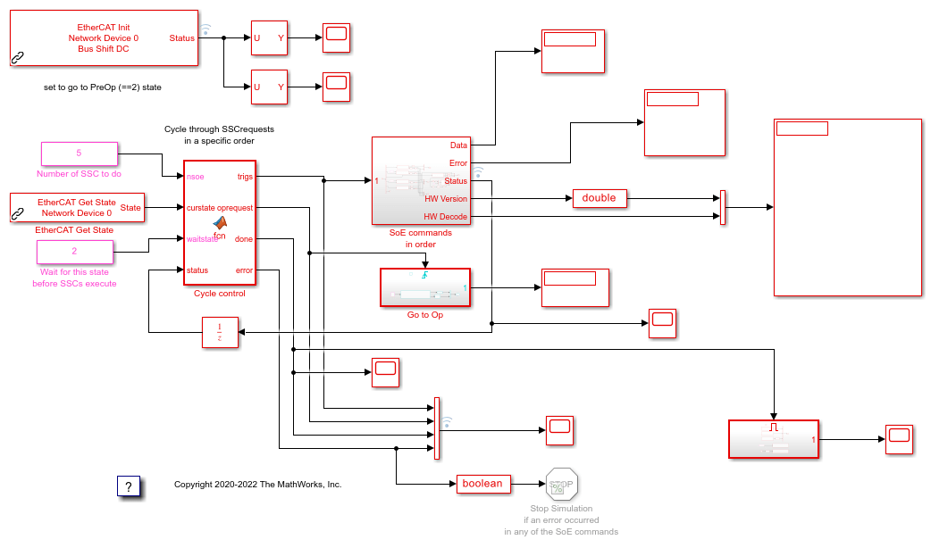
Figure 1: EtherCAT model for sequencing through SoE/SSC commands after pausing initialization at PreOp state
Configure the Model
Open the parameter dialog for the EtherCAT Init block and observe the pre-configured values. The EtherCAT subordinate devices that are daisy chained together with Ethernet cable is a Device, also referred to as an EtherCAT network. The Device Index selects one such chained EtherCAT network. The Ethernet Port Number identifies which Ethernet port to use to access that Device. The EtherCAT Init block connects these two so that other EtherCAT blocks use the Device Index to communicate with the subordinate devices on that EtherCAT network.
If you only have one connected network of EtherCAT subordinate devices, and you have only reserved one Ethernet port with the Ethernet configuration tool, use Device Index = 0 and Ethernet Port Number = 1.
Create an ENI file for a Different SoE drive
If you need to create a new ENI file you need to use a third-party EtherCAT configurator such as TwinCAT 3 from Beckhoff that you install on a development computer. The EtherCAT configuration (ENI) file preconfigured for this model is BeckDrive_1ms.xml.
Each ENI file is specific to the exact network setup for which it was created (for example, the network discovered in step 1 of the configuration file creation process). The configuration file provided for this example is valid if and only if the EtherCAT network consists of one AX5103 drive. If you have a different EtherCAT drive this example still works, but you need to create a new ENI file that uses your drive.
For an overview of the process for creating an ENI file, see Configure EtherCAT Network by Using TwinCAT 3.
If you use a different drive, you need to consult the manual for your devices and find the SoE mapping. Using that mapping, you need to change the SSC commands in the SoE commands in order subsystem to use objects on your drive.
Build, Download, and Run the Model
To build, download, and run the model:
In the Simulink Editor, from the targets list on the Real-Time tab, select the target computer on which to run the real-time application.
Click Run on Target.
If you open the two scopes by double clicking each, the data is relayed from the target back to the development computer and displayed.
The model is preconfigured to run for 15 seconds. If you want to run the model longer, pull down the Run on Target menu and change the number on the bottom line. Press the green arrow to configure, build, and run.
Display the Target Computer Data
If you run the model using the Run on Target button, external mode is connected and you can double click the scope blocks and see the data on the development computer. The Display blocks also work.
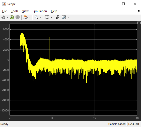
When using Run on Target, Scope shows the DC timing error between the main device code on the target and the first DC enabled subordinate device. Since the error is returned as nanoseconds, this graph shows that the timing difference settles down to the order of 3-5 microseconds (3000 to 5000 nanoseconds) difference between the DC enabled subordinate devices and the target machine running the code. The residual scatter just reflects task scheduling variability in the target computer RTOS.
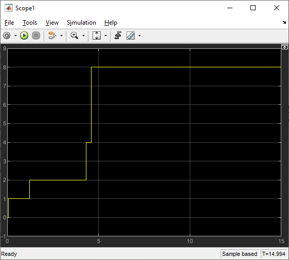
Scope1 shows the progression of EtherCAT states, from idle to Init to PreOp, SafeOp and finally Op state. SafeOp is only entered briefly and only shows up as the value 4 for a few time steps before the switch to Op state. Since this model uses the distributed clocks mechanism, the switch to Op state only occurs once the timing error settles down.
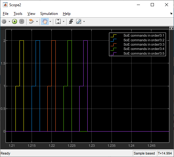
Scope2 shows the status outputs of the 5 async SDO blocks inside the subsystem. Each SDO block is enabled to write for one time step. The block switches to status = 1 (busy) for a few time steps. On successful completion status = 2 (done), the block switches for one time step. If a block encounters an error, the block switches to status = 3 (error) for one time step. On an error, the Cycle control embedded MATLAB code block stops the sequence and sets the error output, which stops the model. In that case, the failing block have output an error code that is displayed on Display1. This display is zoomed into the interval just after state went to PreOp (=2) state.

Scope4 shows several of the outputs from the Cycle control block. The first 5 are the enable signals, made true one at a time by Cycle control. The oprequest output is true for one time step to trigger the request to proceed to Op state. This display is zoomed in to the same interval as in Scope2.
When all of the requested SSC commands are complete and the state has progressed to Op state, the done signal is set to true for the remainder of execution. The rest of your model goes into the Op State Model subsystem.
If you need a different number of SSC commands to execute before Op state, you need to edit the Cycle control embedded MATLAB code block and modify the persistent array that is currently sized to have length 10, which is larger than the number of SSC commands being requested.
If you run the model from the command line, you can use the Data Inspector, accessible from the toolstrip, to view any signal that has been tagged to log with the Log Selected Signals selection found by right clicking on the signal. Those are marked with the dot with two arcs above it in the model editor.
See Also
bdclose(model);