Main Content

predict

Predict responses of censored linear regression model

Since R2025a

    Description

    ypred = predict(mdl,Xnew) returns the predicted response values of the censored linear regression model mdl to the points in Xnew.

    example

    [ypred,yci] = predict(mdl,Xnew) also returns confidence intervals for the responses at Xnew.

    [___] = predict(mdl,Xnew,Name=Value) specifies additional options using one or more name-value arguments. For example, you can specify the significance level of the confidence interval and the prediction type.

    example

    Examples

    collapse all

    Load the readmissiontimes sample data.

    load readmissiontimes

    The variables Age and ReadmissionTime contain data for patient age and time of readmission. The Censored variable contains censoring information for ReadmissionTime.

    Save Age and ReadmissionTime in a table, and fit a censored linear regression model to the data.

    tbl = table(Age,ReadmissionTime,VariableNames=["Age","Time"]);
    mdl = fitlmcens(tbl,Censoring=Censored);

    mdl is a CensoredLinearModel object that contains the results of fitting a linear model to the censored data.

    Generate new predictor data for patient age, and predict response values from the new data.

    Age_New = 25:50;
    Time_New = predict(mdl,Age_New');

    Plot the original responses and the predicted responses to see how they differ.

    plot(Age,ReadmissionTime,"o",Age_New,Time_New,"-")
    legend("Data","Predictions")
    xlabel("Age")
    ylabel("Time")

    Figure contains an axes object. The axes object with xlabel Age, ylabel Time contains 2 objects of type line. One or more of the lines displays its values using only markers These objects represent Data, Predictions.

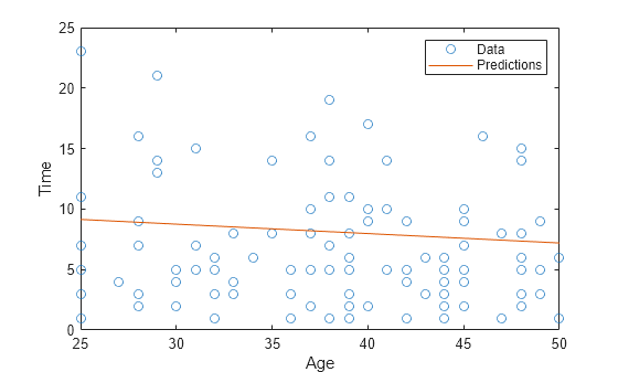
    The plot shows that the predicted responses go through the bulk of the data.

    Load the readmissiontimes sample data.

    load readmissiontimes

    The variables Age and ReadmissionTime contain data for patient age and time of readmission. The Censored variable contains censoring information for ReadmissionTime.

    Save Age and ReadmissionTime in a table, and fit a censored linear regression model to the data.

    tbl = table(Age,ReadmissionTime);
    mdl = fitlmcens(tbl,Censoring=Censored);

    mdl is a CensoredLinearModel object that contains the results of fitting a linear model to the censored data.

    Generate new data for patient age, and calculate simultaneous confidence bounds for the observed data.

    Age_New = 25:50;
    [t,t_ci] = predict(mdl,Age_New',Simultaneous=true,Prediction="observation");

    Plot the responses together with the predicted responses.

    plot(Age,ReadmissionTime,"o",Age_New,t,"-")
    hold on
    plot(Age_New,t_ci(:,1),"--r",Age_New,t_ci(:,2),"--r")
    legend("Data","Predictions","Confidence bounds")
    xlabel("Age")
    ylabel("Time")

    Figure contains an axes object. The axes object with xlabel Age, ylabel Time contains 4 objects of type line. One or more of the lines displays its values using only markers These objects represent Data, Predictions, Confidence bounds.

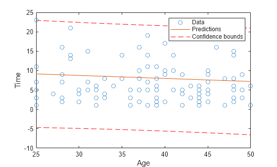
    The plot shows that the observed data falls within the confidence bounds.

    Input Arguments

    collapse all

    Censored linear regression model, specified as a CensoredLinearModel object created using fitlmcens, or a CompactCensoredLinearModel object created using fitlmcens and compact.

    New predictor input values, specified as a table or matrix. Each row of Xnew corresponds to one observation, and each column corresponds to one variable.

    • If Xnew is a table, it must contain predictors that have the same names as predictors in the PredictorNames property of mdl.

    • If Xnew is a matrix, it must have the same number of variables (columns) in the same order as the predictor input used to create mdl. All variables used to create mdl must be numeric. To treat numerical predictors as categorical, specify the predictors using the CategoricalVars name-value argument when you create mdl.

    Note that Xnew must also contain any predictor variables not used as predictors in the fitted model.

    Data Types: single | double | table

    Name-Value Arguments

    collapse all

    Specify optional pairs of arguments as Name1=Value1,...,NameN=ValueN, where Name is the argument name and Value is the corresponding value. Name-value arguments must appear after other arguments, but the order of the pairs does not matter.

    Example: [ypred,yci] = predict(mdl,Xnew,Alpha=0.01,Simultaneous=true) returns the confidence interval yci with a 99% confidence level, and calculates the confidence bounds simultaneously for all predictor values.

    Significance level for the confidence interval, specified as a numeric value in the range [0,1]. The confidence level of yci is equal to 100(1 – Alpha)%. Alpha is the probability that the confidence interval does not contain the true value.

    Example: Alpha=0.01

    Data Types: single | double

    Prediction type, specified as "curve" or "observation".

    A regression model for the predictor variables X and the response variable y has the form

    y = f(X) + ε,

    where f is a fitted regression function and ε is a random noise term.

    • If Prediction is "curve", then the function predicts confidence bounds for f(Xnew), the fitted responses at Xnew.

    • If Prediction is "observation", then the function predicts confidence bounds for y, the response observations at Xnew.

    The bounds for y are wider than the bounds for f(X) because of the additional variability of the noise term.

    Example: Prediction="observation"

    Data Types: string | char

    Flag to compute simultaneous confidence bounds, specified as a numeric or logical 1 (true) or 0 (false).

    • truepredict calculates confidence bounds for the curve of response values corresponding to all predictor values in Xnew, using Schefféʼs method. The range between the upper and lower bounds contains the curve that consists of true response values with 100(1 – α)% confidence.

    • falsepredict calculates confidence bounds for the response value at each observation in Xnew. The confidence interval for a response value at a specific predictor value contains the true response value with 100(1 – α)% confidence.

    With simultaneous bounds, the entire curve of true response values is within the bounds at high confidence. By contrast, nonsimultaneous bounds require only the response value at a single predictor value to be within the bounds at high confidence. Therefore, simultaneous bounds are wider than nonsimultaneous bounds.

    Example: Simultaneous=true

    Output Arguments

    collapse all

    Predicted response values evaluated at Xnew, returned as a numeric vector.

    Confidence intervals for the responses, returned as a two-column matrix in which each row provides one interval. The meaning of the confidence interval depends on the settings of the name-value arguments Alpha, Prediction, and Simultaneous.

    Alternative Functionality

    • The feval function returns the same predictions as the predict function. The feval function can take multiple input arguments, with one input for each predictor variable, which is simpler to use with a model created from a table or dataset array. Note that feval does not give confidence intervals on its predictions.

    • The random function returns predictions with added noise.

    • Use the plotSlice function to create a figure that contains a series of plots, each representing a slice through the predicted regression surface. Each plot shows the fitted response values as a function of a single predictor variable, with the other predictor variables held constant.

    Version History

    Introduced in R2025a