chebyshevT

Chebyshev polynomials of the first kind

Syntax

chebyshevT(n,x)

Description

chebyshevT(n,x) represents the nth degree Chebyshev polynomial of the first kind at the point x.

Examples

First Five Chebyshev Polynomials of the First Kind

Find the first five Chebyshev polynomials of the first kind for the variable x.

syms x
chebyshevT([0, 1, 2, 3, 4], x)

ans =
[ 1, x, 2*x^2 - 1, 4*x^3 - 3*x, 8*x^4 - 8*x^2 + 1]

Chebyshev Polynomials for Numeric and Symbolic Arguments

Depending on its arguments, chebyshevT returns floating-point or exact symbolic results.

Find the value of the fifth-degree Chebyshev polynomial of the first kind at these points. Because these numbers are not symbolic objects, chebyshevT returns floating-point results.

chebyshevT(5, [1/6, 1/4, 1/3, 1/2, 2/3, 3/4])

ans =
    0.7428    0.9531    0.9918    0.5000   -0.4856   -0.8906

Find the value of the fifth-degree Chebyshev polynomial of the first kind for the same numbers converted to symbolic objects. For symbolic numbers, chebyshevT returns exact symbolic results.

chebyshevT(5, sym([1/6, 1/4, 1/3, 1/2, 2/3, 3/4]))

ans =
[ 361/486, 61/64, 241/243, 1/2, -118/243, -57/64]

Evaluate Chebyshev Polynomials with Floating-Point Numbers

Floating-point evaluation of Chebyshev polynomials by direct calls of chebyshevT is numerically stable. However, first computing the polynomial using a symbolic variable, and then substituting variable-precision values into this expression can be numerically unstable.

Find the value of the 500th-degree Chebyshev polynomial of the first kind at 1/3 and vpa(1/3). Floating-point evaluation is numerically stable.

chebyshevT(500, 1/3)
chebyshevT(500, vpa(1/3))

ans =
    0.9631
 
ans =
0.963114126817085233778571286718

Now, find the symbolic polynomial T500 = chebyshevT(500, x), and substitute x = vpa(1/3) into the result. This approach is numerically unstable.

syms x
T500 = chebyshevT(500, x);
subs(T500, x, vpa(1/3))

ans =
-3293905791337500897482813472768.0

Approximate the polynomial coefficients by using vpa, and then substitute x = sym(1/3) into the result. This approach is also numerically unstable.

subs(vpa(T500), x, sym(1/3))

ans =
1202292431349342132757038366720.0

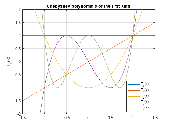
Plot Chebyshev Polynomials of the First Kind

Plot the first five Chebyshev polynomials of the first kind.

syms x y
fplot(chebyshevT(0:4,x))
axis([-1.5 1.5 -2 2])
grid on

ylabel('T_n(x)')
legend('T_0(x)','T_1(x)','T_2(x)','T_3(x)','T_4(x)','Location','Best')
title('Chebyshev polynomials of the first kind')

Input Arguments

n — Degree of polynomial

nonnegative integer | symbolic variable | symbolic expression | symbolic function | vector | matrix

Degree of the polynomial, specified as a nonnegative integer, symbolic variable, expression, or function, or as a vector or matrix of numbers, symbolic numbers, variables, expressions, or functions.

x — Evaluation point

number | symbolic number | symbolic variable | symbolic expression | symbolic function | vector | matrix

Evaluation point, specified as a number, symbolic number, variable, expression, or function, or as a vector or matrix of numbers, symbolic numbers, variables, expressions, or functions.

More About

Chebyshev Polynomials of the First Kind

• Chebyshev polynomials of the first kind are defined as T_n(x) = cos(n*arccos(x)).

  These polynomials satisfy the recursion formula

  $$T\left(0,x\right)=1,T\left(1,x\right)=x,T\left(n,x\right)=2xT\left(n-1,x\right)-T\left(n-2,x\right)$$

• Chebyshev polynomials of the first kind are orthogonal on the interval -1 ≤ x ≤ 1 with respect to the weight function $$w\left(x\right)=\frac{1}{\sqrt{1-x^2}}$$.

  $${\displaystyle \underset{-1}{\overset{1}{\int }}\frac{T(n,x)T(m,x)}{\sqrt{1-x^2}}dx}=\{\begin{array}{cc}0& \text{if }n\ne m\\ \pi & \text{if }n=m=0\\ \frac{\pi }{2}& \text{if }n=m\ne 0.\end{array}$$

• Chebyshev polynomials of the first kind are special cases of the Jacobi polynomials

  $$T\left(n,x\right)=\frac{2^{2n}{\left(n!\right)}^2}{\left(2n\right)!}P\left(n,-\frac{1}{2},-\frac{1}{2},x\right)$$

  and Gegenbauer polynomials

  $$T\left(n,x\right)=\{\begin{array}{cc}\frac{1}{2}\underset{a\to 0}{\lim }\frac{n+a}{a}G\left(n,a,x\right)& \text{if }n\ne 0\\ \underset{a\to 0}{\lim }G\left(0,a,x\right)=1& \text{if }n=0\end{array}$$

Tips

• chebyshevT returns floating-point results for numeric arguments that are not symbolic objects.

• chebyshevT acts element-wise on nonscalar inputs.

• At least one input argument must be a scalar or both arguments must be vectors or matrices of the same size. If one input argument is a scalar and the other one is a vector or a matrix, then chebyshevT expands the scalar into a vector or matrix of the same size as the other argument with all elements equal to that scalar.

References

[1] Hochstrasser, U. W. “Orthogonal Polynomials.” Handbook of Mathematical Functions with Formulas, Graphs, and Mathematical Tables. (M. Abramowitz and I. A. Stegun, eds.). New York: Dover, 1972.

[2] Cohl, Howard S., and Connor MacKenzie. “Generalizations and Specializations of Generating Functions for Jacobi, Gegenbauer, Chebyshev and Legendre Polynomials with Definite Integrals.” Journal of Classical Analysis, no. 1 (2013): 17–33. https://doi.org/10.7153/jca-03-02.

Version History

Introduced in R2014b