Reconstruct 3-D Scenes and Synthesize Novel Views Using Neural Radiance Field Model

This example shows you how to reconstruct a 3-D representation of a scene as a dense, photorealistic point cloud from a sequence of 2-D RGB images, and synthesize novel views of the scene, by using the Nerfacto Neural Radiance Field (NeRF) model [1] from the Nerfstudio library [2].

A NeRF model represents complex 3-D scenes by implicitly encoding scene geometry and appearance within neural network parameters. When you train the model using the trainNerfacto function, the model first samples a batch of rays that consist of multiple spatial locations and viewing directions. The neural network then predicts the color and density at 3-D points along each ray, and the NeRF model uses volumetric rendering to project the output colors and densities onto an image. The model calculates the training loss by comparing the image pixels of the rendered image against the captured images in the training data.

This example consists of these processes:

• Generate Point Cloud and Novel Views with Pretrained NeRF Model.

• Train NeRF Model and Write Novel Views to Image Files.

• Generate Smooth Trajectories from Densely Sampled Novel Views.

Prerequisites

• This example requires the Computer Vision Toolbox™ Interface for Nerfstudio Library, which you can install using the Add-On Explorer. For more information about installing add-ons, see Get and Manage Add-Ons.

• The Computer Vision Toolbox Interface for Nerfstudio Library requires a Deep Learning Toolbox™ license, a Computer Vision Toolbox license, a Parallel Computing Toolbox™ license, and a supported GPU device. For more information on the computing requirements, see GPU Computing Requirements (Parallel Computing Toolbox)

Generate Point Cloud and Novel Views Using Pretrained NeRF Model

Reconstruct a 3-D representation of a scene as a dense, photorealistic point cloud, and synthesize novel views of the scene, using a pretrained NeRF model.

Download Pretrained NeRF Model

The tum_rgbd_nerfacto.zip file contains the trainedNerfactoTUMRGBD folder. The folder contains the saved-nerfacto-tum-rgbd.mat supporting file, which contains a nerfacto object that has been trained on a sequence of indoor images from the TUM RGB-D data set [3], and the nerfactoModelFolder folder, which contains the data and configuration files required for the Nerfstudio Library to load and execute the trained model.

Download and extract tum_rgbd_nerfacto.zip.

if ~exist("tum_rgbd_nerfacto.zip","file")
    websave("tum_rgbd_nerfacto.zip","https://ssd.mathworks.com/supportfiles/3DReconstruction/tum_rgbd_nerfacto.zip");
    unzip("tum_rgbd_nerfacto.zip",pwd);
end

Load Pretrained nerfacto Object into Workspace

Specify the path to the folder containing the saved-nerfacto-tum-rgbd MAT file, and then load the pretrained nerfacto object into the workspace.

modelRoot = fullfile(pwd,"trainedNerfactoTUMRGBD");
load(fullfile(modelRoot,"saved-nerfacto-tum-rgbd.mat"))

Warning: The model folder for the nerfacto object could not be loaded. Update the model folder location using the <a href="matlab:doc('changePath')">changePath</a> method.
  '\\mathworks\devel\sandbox\user\Shared\EX_25b\EX_nerfacto_feature\train_nerfacto_small'

MATLAB® displays a warning when you first load the pretrained nerfacto object into the workspace because the path to the model folder associated with the object, nerfactoModelFolder, changes when you extract the nerfacto_saved_model.zip.

To resolve this issue, use the changePath function to update the ModelFolder property of the trained nerfacto object to the current path of nerfactoModelFolder. This process can take a few minutes.

nerf = changePath(nerf,fullfile(modelRoot,"nerfactoModelFolder"));

Changing nerfacto object model folder path.
nerfacto object model folder path change complete.

Display the nerfacto object properties to verify that the ModelFolder property is set to the current path of nerfactoModelFolder on your system.

disp(nerf)

  nerfacto with properties:

      ModelFolder: "/home/user/Documents/MATLAB/ExampleManager/user.Bdoc.Nov-13/vision-ex23411435/trainedNerfactoTUMRGBD/nerfactoModelFolder"
    MaxIterations: 30000
       Intrinsics: [1×1 cameraIntrinsics]

Generate Point Cloud Using Pretrained NeRF Model

Use the generatePointCloud function to generate a dense, colored point cloud of the scene. Set the maximum number of points in the point cloud to 100,000 by specifying the MaxNumPoints name-value argument. This value achieves a balance between the quality of the point cloud, the computing time, and storage space.

ptCloud = generatePointCloud(nerf,MaxNumPoints=100000);

Generating point cloud from nerfacto object.
Loading latest checkpoint from load_dir
Setting up the Nerfstudio pipeline...
[06:59:00 PM] Auto image downscale factor of 1                                              nerfstudio_dataparser.py:484
Setting up training dataset...
Caching all 104 images.
Loading latest checkpoint from load_dir
nerfacto object point cloud generation complete.

Visualize the point cloud by using the pcshow function, and specify the vertical axis and vertical axis direction to match the coordinate system of the TUM RGB-D data set used to train the nerfacto object. Modify the view of the point cloud visualization to focus on the scene region of interest by specifying the of low-level camera properties of the axes object. For more information on configuring these properties, see Low-Level Camera Properties

figure
ax = pcshow(ptCloud,VerticalAxis="y",VerticalAxisDir="down");
ax.CameraPosition = [-1.5185 -6.5178 -11.9106];
ax.CameraUpVector = [0.0520 -0.8878 0.4572];
ax.CameraViewAngle = 15;
xlabel("X")
ylabel("Y")
zlabel("Z")
title("Point Cloud from NeRF")

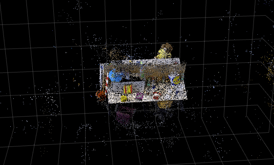
Tip: You can use the pcdenoise function to clean up the outliers and noise in the point cloud.

Generate Novel Views Using Pretrained NeRF Model

This example contains a set of predefined camera poses that are stored as an array of rigidtform3d objects in the camera-poses-tum.mat file. These represent the position and orientation of the camera in the 3-D world coordinate system of the scene.

Load the camera-poses-tum.mat file into workspace, which contains the camera poses camPoses.

load("camera-poses-tum.mat","camPoses");

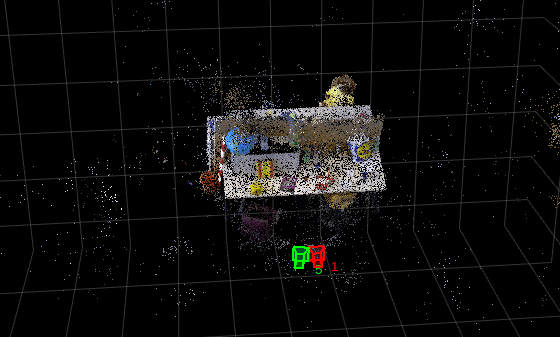
Display the first and fifth camera poses on the point cloud visualization by using the plotCamera function. Observe that these poses point the cameras at the desk, which has a blue globe on it.

hold on
plotCamera(AbsolutePose=camPoses(1),Size=0.1,Label="1",Color=[1 0 0],Parent=ax)
plotCamera(AbsolutePose=camPoses(5),Size=0.1,Label="5",Color=[0 1 0],Parent=ax)
hold off

Generate the views captured by the first and fifth camera poses by using the generateViews function.

images = generateViews(nerf,camPoses([1 5]));

Generating views from nerfacto object.
Loading latest checkpoint from load_dir
nerfacto object view generation complete.

Tip: If you want to generate a large number of novel views, use the writeViews function instead of generateViews to avoid an out-of-memory error.

Display the generated images. The images show the globe on the desk that is present in the point cloud.

figure
montage(images,BorderSize=[2 2])
title("Rendered Images from Trained NeRF")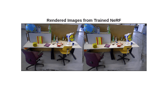

Train NeRF Model and Write Novel Views to Image Files

You can use image data of a scene to train a NeRF model, and then use the trained model to synthesize novel views of the scene.

Training Data Requirements

To train a NeRF model on a scene, your training set must contain:

• At least 100 images of the scene from multiple overlapping views of the region of interest.

• Camera poses associated with each image.

• Intrinsic parameters of camera used to capture the images.

To calculate the intrinsic parameters of camera through calibration, use the Camera Calibrator app. For information on estimating camera poses and related geometric information, see the Structure from Motion from Multiple Views example.

After you train the NeRF model on a scene, you can use the model to generate realistic images of this scene from other viewpoints, and create dense colored point clouds representation of the scene.

Download Training Data

The tum_rgbd_nerfacto.zip file contains the sfmTrainingDataTUMRGBD folder. The folder contains the cameraInfo.mat file which contains the camera poses associated with each image and the intrinsic parameter of camera, and the images folder which contains indoor images from the TUM RGB-D dataset, which is the same dataset used to train the pretrained nerfacto object in the previous section.

Download and extract tum_rgbd_nerfacto.zip.

if ~exist("tum_rgbd_data.zip","file")
    websave("tum_rgbd_data.zip","https://ssd.mathworks.com/supportfiles/3DReconstruction/tum_rgbd_data.zip");
    unzip(fullfile("tum_rgbd_data.zip"),pwd);
end

Set Up Training Data

Specify the path to the images folder, and then create an imageDatastore object using the path.

trainingImageFolder = fullfile("sfmTrainingDataTUMRGBD","images");
imds = imageDatastore(trainingImageFolder);
disp("Number of images: " + length(imds.Files))

Number of images: 104

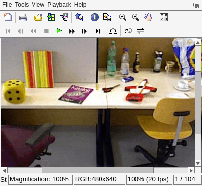
Show the first training image.

figure
sampleTrainingImage = preview(imds);
imshow(sampleTrainingImage)
title("Sample Training Image")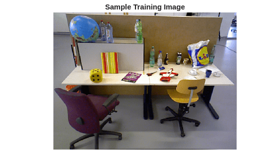

Load the camera poses corresponding to the training images, and the intrinsic parameters of the camera used to capture the images.

camInfo = load(fullfile("sfmTrainingDataTUMRGBD","cameraInfo.mat"));
trainIntrinsics = camInfo.intrinsics;
trainPoses = camInfo.cameraPoses;

Display the camera poses. Observe that there are 104 camera poses, which corresponds to the 104 training images in the image datastore imds.

disp(trainPoses)

  1×104 rigidtform3d array with properties:

    Dimensionality
    Translation
    R
    A

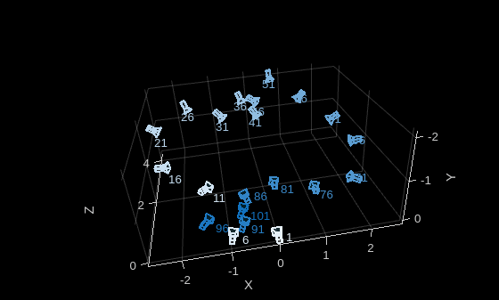
Plot the camera positions of the training images.

figure
pcshow([NaN NaN NaN],VerticalAxis="y",VerticalAxisDir="down");
xlabel("X")
ylabel("Y")
zlabel("Z")
hold on

% Plot only every fifth camera position for a more legible visualization
cameraIds = 1:5:numel(trainPoses);
camerasToPlot = trainPoses(1:5:end);
colors = sky(length(camerasToPlot));
for i = 1:length(camerasToPlot)
    plotCamera(camerasToPlot(i),Size=0.1,Label=cameraIds(i),Color=colors(i,:),Opacity=0.1);
end

hold off

Train NeRF Model

Use the trainNerfacto function to create and train a NeRF model on the training images across up to 10,000 iterations. Store intermediate model checkpoints and configurations in the sfmTrainingDataTUMRGBD folder.

To perform training, set doTraining to true. Training requires about 60 minutes on a Linux machine with an NVIDIA GeForce RTX 3090 GPU that has 24 GB of memory.

doTraining = false;
if doTraining
    trainFolder = fullfile(pwd,"sfmTrainingDataTUMRGBD");
    nerf = trainNerfacto(imds,trainPoses,trainIntrinsics,trainFolder,MaxIterations=10000);
end

Write Novel Views from Trained NeRF Model to Image Files

Write the views captured by the first 20 camera poses to a local folder, generatedTrainingViewsGT, by using the writeViews function.

imdsGen = writeViews(nerf,trainPoses(1:20),"generatedTrainingViewsGT");

Generating views from nerfacto object.
Loading latest checkpoint from load_dir
nerfacto object view generation complete.

Display a side-by-side comparison between the training images and the generated images of the scene at a camera pose. Each comparison includes these metrics that quantify the similarity between the training images and the generated images:

• Structural Similarity Index Metrics (SSIM) — Value in the range [0,1], where a value of 1 indicates the perfect similarity.

• Peak Signal-to-Noise Ratio (PSNR) — Values are in decibels, where higher values indicate better similarity.

imageIdx selects the camera pose to compare.

numImg = numel(imdsGen.Files);
imageIdx = 10;

% Load image generated by the trained NeRF
imageGen = readimage(imdsGen,imageIdx);

% Load the corresponding real image used in training
imageReal = readimage(imds,imageIdx);

% Compute image similarity metrics - SSIM and PSNR
ssimVal = ssim(rgb2gray(imageGen),rgb2gray(imageReal));
psnrVal = psnr(imageGen,imageReal);

% Visualize the images and their similarity maps
figure
montage({imageReal,imageGen},BorderSize=[2 2])
title("[Real | Generated] Image " + imageIdx + ": SSIM=" + num2str(ssimVal,2) + "; PSNR=" + num2str(psnrVal,4))
truesize;

Tips to Improve Training Results

Although the generated images are photorealistic, there are minor differences in the image texture and high-frequency details between the generated images and the training images. To achieve better quality results:

• Capture a larger set of high resolution images.

• Ensure the image set has good lighting.

• Ensure the image set has no motion blur or moving objects.

• Train the nerfacto object with a higher number of maximum training iterations (at the cost of longer computation time).

Generate Smooth Trajectories from Densely Sampled Novel Views

After training a NeRF model using a set of images and their camera parameters, you can render novel viewpoints that are not part of the original data set. This example shows you how to generate a smooth video of the scene by sampling a dense sequence of virtual camera poses along the same trajectory as the training set of images. Because the NeRF model represents scene appearance and geometry as a continuous function, the model naturally supports high-framerate rendering and smooth interpolation between viewpoints, even when the training images are sparsely distributed. The result is a high-quality visualization of the reconstructed scene in the form of a high-framerate video. Such high-framerate videos are useful for visually inspecting 3-D reconstructions, generating walkthroughs of a scene, or augmenting data sets with additional rendered views for downstream computer vision tasks.

Visualize Original Image Sequence

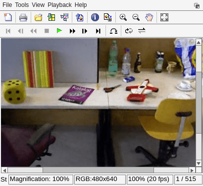
Visualize the original set of images used to train the NeRF model, and save the video as imageSequenceTrainVideo.avi. Display the video, and note the gaps between frames.

outputVideo = VideoWriter("imageSequenceTrainVideo.avi");
outputVideo.FrameRate = 20;
open(outputVideo);

reset(imds);
while hasdata(imds)
    I = read(imds);
    writeVideo(outputVideo,I);
end

close(outputVideo);

% Launch the video player
implay("imageSequenceTrainVideo.avi");

Interpolate Two Camera Poses to Create Intermediate Cameras

The interp function performs spherical-linear interpolation (SLERP) on the rotational component and linear interpolation on the translational component of camera poses. This enables interpolation between successive camera poses, generating a continuous and smooth virtual trajectory that preserves proper rotational geometry and avoids artifacts such as axis flips or gimbal-lock singularities [4].

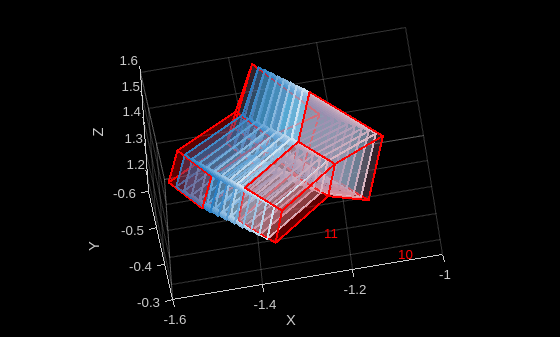
Insert 10 intermediate camera poses along a segment of the camera path between 2 original camera poses.

camIndex = 10;
numPoses = 10;
pose1 = se3(trainPoses(camIndex));
pose2 = se3(trainPoses(camIndex + 1));
interPoses = interp(pose1,pose2,numPoses);
interPoses = rigidtform3d(interPoses);

Build a camera table with a custom colormap for the interpolated cameras.

interpCamColors = sky(length(interPoses));
cameraTable = table(interPoses(:),interpCamColors,VariableNames=["AbsolutePose","Color"]);

Visualize the cameras. Display the original camera poses in red and the interpolated cameras using a sky-blue palette.

figure
pcshow([NaN NaN NaN],VerticalAxis="y",VerticalAxisDir="down");
xlabel("X")
ylabel("Y")
zlabel("Z")
hold on
plotCamera(cameraTable,Size=0.1)
plotCamera(trainPoses(camIndex),Size=0.1,Color="red",Label=num2str(camIndex));
plotCamera(trainPoses(camIndex+1),Size=0.1,Color="red",Label=num2str(camIndex+1));
hold off

Use All Training Camera Poses to Generate Complete, Dense, Virtual Trajectory

Create new virtual cameras by interpolating five intermediate poses between each of consecutive training camera poses.

numPoses = 5;
denseCameraPoses = cell(length(trainPoses)-1,1);
for camIndex = 1:length(trainPoses)-1
    pose1 = se3(trainPoses(camIndex));
    pose2 = se3(trainPoses(camIndex+1));
    interPoses = interp(pose1,pose2,numPoses);
    interPoses = rigidtform3d(interPoses);
    denseCameraPoses{camIndex} = interPoses;
end
denseCameraPoses = cat(1,[denseCameraPoses{:}]);

Render Novel Views from Interpolated Camera Poses

Use the NeRF model to synthesize novel views along the virtual trajectory. Each intermediate pose specifies a virtual position and orientation for the camera in the scene, and the NeRF rendering function evaluates the learned radiance field to generate a corresponding RGB image.

Write the images to a local folder, generatedDenseViews, by using the writeViews function. This requires around 30 minutes on a Linux machine with an NVIDIA GeForce RTX 3090 GPU that has 24 GB of memory.

imdsDense = writeViews(nerf,denseCameraPoses,"generatedDenseViews");

Generating views from nerfacto object.
Loading latest checkpoint from load_dir
nerfacto object view generation complete.

Visualize Generated Dense Image Sequence

Visualize the generated trajectory as a video and save it as imageSequenceDenseVideo.avi. Display the video. Note that playback is considerably smoother compared to the original sequence imageSequenceTrainVideo.avi. Because the original video was captured in casual setting using a handheld camera, you can observe several artifacts in the visualization of the generated trajectory. For information on how to improve the quality of a generated image sequence, see Tips to Improve Training Results.

outputVideo = VideoWriter("imageSequenceDenseVideo.avi");
outputVideo.FrameRate = 20;
open(outputVideo);

reset(imdsDense);
while hasdata(imdsDense)
    I = read(imdsDense);
    writeVideo(outputVideo,I);
end

close(outputVideo);

% Launch the video player
implay("imageSequenceDenseVideo.avi");

References

[1] Mildenhall, Ben, Pratul P. Srinivasan, Matthew Tancik, Jonathan T. Barron, Ravi Ramamoorthi, and Ren Ng. "NeRF: Representing Scenes as Neural Radiance Fields for View Synthesis." In Computer Vision - ECCV 2020, edited by Andrea Vedaldi, Horst Bischof, Thomas Brox, and Jan-Michael Frahm. Springer International Publishing, 2020. https://doi.org/10.1007/978-3-030-58452-8_24.

[2] Tancik, Matthew, Ethan Weber, Evonne Ng, et al. “Nerfstudio: A Modular Framework for Neural Radiance Field Development.” Special Interest Group on Computer Graphics and Interactive Techniques Conference Proceedings, ACM, July 23, 2023, 1–12. https://doi.org/10.1145/3588432.3591516.

[3] Sturm, Jürgen, Nikolas Engelhard, Felix Endres, Wolfram Burgard, and Daniel Cremers. “A Benchmark for the Evaluation of RGB-D SLAM Systems.” 2012 IEEE/RSJ International Conference on Intelligent Robots and Systems, October 2012, 573–80. https://doi.org/10.1109/IROS.2012.6385773.

[4] Shoemake, Ken. “Animating Rotation with Quaternion Curves.” ACM SIGGRAPH Computer Graphics 19, no. 3 (1985): 245–54. https://doi.org/10.1145/325165.325242.