Select Detection Approach for Visual Inspection

R2026b

The Visual Inspection Toolbox™ provides four approaches for detecting, localizing, and quantifying objects and defects in inspection images: anomaly detection, shape matching, object detection, and object counting. The best approach for your application depends primarily on three factors: how well you can characterize the objects or defects of interest in advance, what data you have available, and what output your inspection decision requires.

Use these guidelines to identify the approach that best matches your application, then follow the corresponding topics and examples for that approach.

Answer These Questions First

To narrow down the approach based on your application and available data, consider these questions in order:

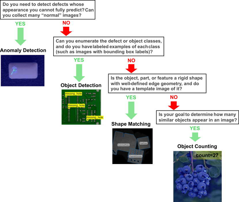
If your inspection task involves more than one of these goals, you can combine approaches. See Combine Approaches in an Inspection Workflow.

Note

If your inspection requires a calibrated dimensional measurement, such as a distance, diameter, or angle, use the caliper and edge-fitting measurement tools, typically after locating the part with shape matching. See Measurement.

Compare Approaches

This table compares the four detection approaches across the criteria that most often determine the best fit for an application.

Comparison of Detection Approaches

Criteria	Anomaly Detection	Shape Matching	Object Detection	Object Counting
Task goal	Detect any deviation from normal appearance, including previously unseen defect types. Typical application examples include: Surface defects (scratches, dents, contamination) Novel failure modes Pass or fail screening	Detect and localize rigid parts with known edge geometry, and aligning images to a reference. Typical application examples include: Part presence and orientation checks Pick-and-place, aligning parts for measurement or downstream inspection	Detect, localize, and classify instances of known object or defect classes. Typical application examples include: Recurring defect types that must be classified, such as PCB defects Multi-class inspection	Count many similar objects in complex scenes Component kitting verification Counting products or parts in dense scenes
Prior knowledge required	What normal parts look like	A template image of each target shape	Representative labeled examples of every class	One or more exemplar patches of the object to count
Training data	Normal images only (one-class learning); optionally a small number of anomalous images (outlier exposure); labeled calibration set for thresholding	None – create a shape model from a single template image (one-shot)	Images with bounding box labels per class; synthetic training data generation supported	None – few-shot exemplars selected at run time
Output	Image-level anomaly score and normal or anomalous classification, plus pixel-level anomaly map	Match locations with class name, score, and subpixel pose (translation, rotation, scale)	Bounding boxes with class labels and confidence scores	Object count and density map
Localization precision	Pixel-level heatmap (approximate region)	Subpixel – suitable for measurement and alignment	Bounding box per instance	Density map; approximate locations
Robustness	Sensitive to imaging changes – consistent lighting and part presentation improve accuracy	Matches on edge orientation, not pixel intensity – robust to illumination changes; handles partial occlusion	Robust to appearance variation covered by training data; tiled training supports small objects in large images	Handles dense, overlapping instances where per-instance detection degrades
Key limitations	Does not identify defect type	Detects only rigid shapes that match the template; not suited to variable-appearance defects	Cannot find defect types absent from training data	Counts one object type per exemplar set; no classification
Speed and hardware	Training: minutes to hours on CPU. Inference: GPU recommended; CPU possible but slower.	No training. Inference: CPU only.	Training: minutes to hours on GPU. Inference: GPU recommended; CPU possible but slower.	No per-class training. Inference: GPU recommended; CPU possible but slower.

Anomaly Detection

Use anomaly detection when you cannot predict every way a part can fail. Anomaly detectors learn the appearance of normal parts and classify test images as normal or anomalous. They also return an anomaly map that highlights regions that differ from normal appearance.

The toolbox provides Student-Teacher, PatchCore, FastFlow, and FCDD anomaly detectors, which differ in training requirements such as supported image sizes, model size, and low-shot support. For a comparison, see Get Started with Anomaly Detection Using Deep Learning. To train, evaluate, and compare detectors interactively, use the Visual Anomaly Detector app.

Use anomaly detection when:

• Defects are rare, subtle, or unpredictable, and new defect modes can appear over the lifetime of the model.

• You have many images of good parts, but anomalous samples are scarce or expensive to collect.

• A pass or fail decision per image, with an approximate defect location, is sufficient.

• Imaging conditions, such as lighting, camera position, and part presentation, are consistent, so that appearance changes indicate true anomalies.

For an example, see Localize Screen Manufacturing Defects Using Student-Teacher Anomaly Detector.

Consider a different approach when:

• The inspection decision depends on the type of defect. In this case, use object detection, or train a defect classification network such as visionTransformer if you have sufficient labeled data for each defect class. For an example, see Classify Defects on Wafer Maps Using Deep Learning.

• The defect is a missing, misplaced, or misoriented part with known geometry. In this case, use shape matching.

To build an anomaly detection data set, collect normal images that span the full range of acceptable variation, such as part-to-part differences, allowed tolerances, and minor lighting drift. Use labeled normal and anomalous images to calibrate the anomaly threshold. Some detectors can also use a small number of real or synthetic anomalous images during training as outlier exposure.

Object Detection

Use object detection when you know the defect or object classes in advance and need to locate and classify each instance. YOLOX detectors return bounding boxes, class labels, and confidence scores for detected objects or defects. To interactively detect objects and analyze detection results, use the Object Detector Analyzer app.

Use object detection when:

• Your defect or target classes are known, visually distinct, and recur often enough to collect labeled examples.

• The inspection decision depends on the defect type — for example, different defect classes require different follow-up actions.

• Defects or objects within a class vary in appearance, size, or orientation in ways that rigid template matching cannot capture.

• You plan to deploy the model outside MATLAB^®. To learn more about deployment options, see Deploy Visual Inspection Code, Models, and Applications.

Consider a different approach when:

• You cannot collect and label enough examples per class, or unknown defect types must also be caught. In this case, use anomaly detection, alone or as a first screen alongside object detection.

• The objects have consistent, rigid shapes and you need pose information rather than a class-labeled bounding box. In this case, use shape matching, which requires no training.

Object detection requires images labeled with bounding boxes for each class. You can use existing labeled data, label images using the Image Labeler app, or generate synthetic training images when labeled data is limited. For industrial defect detection, see Detect Defects on Printed Circuit Boards Using YOLOX Network. For synthetic training data, see Train YOLOX Object Detector Using Synthetic Data.

To get started, see Detect Objects Using YOLOX Deep Learning Network.

Shape Matching

Use shape matching to detect and localize rigid parts or features with known geometry. Shape matching requires a template image, not training data, and returns the location, score, and subpixel pose of each match. Because shape matching uses edge orientation rather than pixel intensity, it is robust to illumination changes and surface reflectance variation, such as on texture-less metallic parts.

Shape matching supports searches for multiple template classes in a single image and can detect partially occluded objects.

Use shape matching when:

• You are detecting, locating, or verifying parts with well-defined, repeatable edge geometry, such as machined or stamped components.

• You have a template image per part class but no training data, or you need deterministic, explainable behavior for process validation.

• You need subpixel pose accuracy — for example, to align images to a reference, position measurement tools for calibrated dimensional inspection, or guide pick-and-place operations.

• Lighting varies between captures, making intensity-based methods unreliable.

For an example, see Detect Industrial Parts Using Multi-Class Shape-Based Matching.

Consider a different approach when:

• The objects or defects belong to known classes, but a single template cannot reliably represent their appearance. In this case, use object detection.

• You are looking for unexpected surface defects or appearance anomalies rather than locating geometric features with a known shape. In this case, use anomaly detection.

Object Counting

Use object counting when the inspection decision is a quantity, such as verifying that a kit contains the correct number of components or counting parts in a bin. The CounTR model uses a few-shot, exemplar-based approach, so you can count similar objects without class-specific training or per-object annotations.

Use object counting when:

• You need to determine the number of similar objects in an image, especially in dense scenes with many instances, overlap, or occlusion, where per-instance detection becomes unreliable.

• The object type varies between inspections, making it impractical to train a dedicated detector for each type because exemplar patches adapt the counter at run time.

Consider a different approach when:

• You also need to classify or localize each instance with a bounding box, and instances are well separated. In this case, a trained YOLOX detector provides boxes you can count and classify.

• You are verifying the presence of a specific small number of rigid parts. In this case, use shape matching to detect each instance and its pose without exemplars.

For an example, see Count Objects Using CounTR Model.

Combine Approaches in an Inspection Procedure

You can combine these approaches in an inspection procedure. For example, you can:

• Locate and align, then inspect — Use shape matching to detect the part and recover its pose, then align the image to a reference and run anomaly detection on the aligned region of interest. Pose normalization tightens the definition of normal appearance and improves anomaly detection accuracy.

• Locate, then measure — Use the pose returned by shape matching to position caliper and edge-fitting measurement tools for calibrated dimensional inspection. For an example, see Automate Calibrated Image Measurement Using Shape Matching.

• Screen, then classify — Use anomaly detection as a broad first screen that catches deviations from normal appearance, then apply a defect classification network or object detector to flagged images to identify known defect types.

• Detect, then count — Use object detection to find regions containing objects of interest, then count within each region, or compare a detector-based count against a CounTR count as a cross-check in dense scenes.