dlidwt

Differentiable inverse discrete wavelet transform

Since R2025a

Syntax

Y = dlidwt(A,D)

Y = dlidwt(A,D,Name=Value)

Description

Y = dlidwt(A,D) returns the inverse discrete wavelet transform (DWT) of the approximation (scaling) coefficients A and detail (wavelet) coefficients D using the Haar wavelet and "reflection" padding at the boundary.

Y = dlidwt(A,D,Name=Value) specifies options using one or more name-value arguments. For example, PaddingMode="zeropad" specifies zero padding at the boundary.

Examples

Deep Learning Inverse Discrete Wavelet Transform

1-D Inverse DWT

Load the wecg signal. The data is arranged as a 2048-by-1 vector. Store the signal in a dlarray with format "TCB".

load wecg
wecgdl = dlarray(wecg,"TCB");

Use dldwt to obtain the full deep learning DWT of the signal using the Haar wavelet down to level 3. Then use wavedec to obtain the DWT of the original signal down to the same level using the same wavelet. Because wavedec uses the global variable managed by dwtmode as the default extension, specify the extension mode as "sym", which is the default extension mode of dldwt.

lev = 3;
wv = "haar";
[At,Dt] = dldwt(wecgdl,Wavelet=wv,Level=lev, ...
    FullTree=true);
[c,l] = wavedec(wecg,lev,wv,Mode="sym");

Use dlidwt to reconstruct the DWT up to level 1, which is equal to the projection onto the scaling space at level 1, one scale coarser than the resolution of the data. The result is a dlarray object in "CBT" format containing the approximation coefficients at level 1. Extract the coefficients from the dlarray object.

reclev = 1;
xrecdl = dlidwt(At,Dt,Wavelet=wv,Level=reclev);
appcf = extractdata(xrecdl);

Use appcoef to obtain the approximation coefficients at the same level.

xrec = appcoef(c,l,wv,reclev,Mode="sym");

Confirm both sets of coefficients are effectively equal.

max(max(appcf(:)-xrec(:)))

ans = 
0

2-D Inverse DWT

Load the xbox image. The image is arranged as a 128-by-128 matrix. Store the image in a dlarray with format "SSCB".

load xbox
xboxdl = dlarray(xbox,"SSCB");

Obtain the full deep learning DWT of the image down to level 4 using the bior4.4 wavelet.

wv = "bior4.4";
lev = 4;
[AI,DI] = dldwt(xboxdl,Wavelet=wv,Level=lev, ...
    FullTree=true);

Use wavedec2 to obtain the DWT of the original image down to the same level using the same wavelet. Because wavedec2 uses the global variable managed by dwtmode as the default extension, you must set that variable to "sym". First save the current extension mode, and then change to symmetric boundary handling.

origMode = dwtmode("status","nodisplay");
dwtmode("sym","nodisplay")
[c,s] = wavedec2(xbox,lev,wv);

Use dlidwt to reconstruct the DWT up to level 1, which is equal to the projection onto the scaling space at level 1, one scale coarser than the resolution of the data. The result is a dlarray object in "SSCB" format containing the approximation coefficients at level 1. Extract the coefficients from the dlarray object.

reclev = 1;
xrecdl2= dlidwt(AI,DI,Wavelet=wv,level=reclev);
appcf2 = extractdata(xrecdl2);

Use appcoef2 to obtain the approximation coefficients at the same level. Then confirm both sets of coefficients are effectively equal.

xrec = appcoef2(c,s,wv,reclev);
max(abs(appcf2(:)-xrec(:)))

ans = 
4.2633e-14

Reset the default extension mode to its original value.

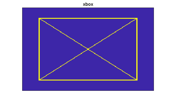
dwtmode(origMode,"nodisplay")

Apply Gains to Multichannel Image

Load the xbox image. The image is a 128-by-128 matrix.

load xbox
imagesc(xbox)
set(gca,'xtick',[])
set(gca,'ytick',[])
title("xbox")

Create a random 2-D multichannel image with five channels. The size of the row and column dimensions are 128. Store the xbox image in the first and fourth channels.

ind1 = 1;
ind2 = 4;
nchan = 5;
img = randn(128,128,nchan);
img(:,:,ind1) = xbox;
img(:,:,ind2) = xbox;

Use dldwt to obtain the full DWT of the multichannel image down to level 4. Because the input is a numeric array, you must specify the data format. Set DataFormat to "SSCB". The output coefficients are unformatted dlarray objects.

lev = 4;
[a,d] = dldwt(img,Level=lev,DataFormat="SSCB",FullTree=true);

Reconstruct the multichannel image up to level 1. For the image in the first channel, apply a gain of 0 to the HH subband at all levels. For the image in the fourth channel, apply a gain of 0 to the HL and LH subbands. A gain is a real-valued scalar between 0 and 1 inclusive. To apply gains to the wavelet subbands of the full DWT, first create an NC-by-3-by-L array of all ones, where NC is the number of channels, and L is the difference between the decomposition level and reconstruction level. The second dimension corresponds to the wavelet subbands in this order: HL, LH, and HH.

recLevel = 1;
diffLevels = lev-recLevel;
dg = ones(nchan,3,diffLevels);

Set the gain of the HH subband at all levels for the image in the first channel to 0.

dg(ind1,3,:) = 0;

Set the gains of the HL and LH subbands at all levels for the image in the fourth channel to 0.

dg(ind2,1:2,:) = 0;

Now apply the gains and reconstruct the image. Because the coefficients are unformatted dlarray objects, set DataFormat to "SSCB".

xrecdl = dlidwt(a,d,Level=recLevel,DetailGain=dg, ...
    DataFormat="SSCB");

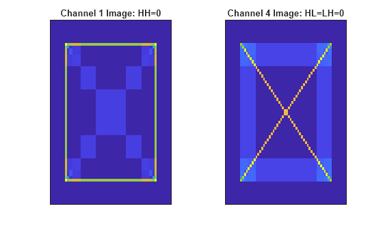
Plot the reconstruction of the first and fourth channels. Recall that the HH subband corresponds to the diagonal details, and the HL and LH subbands correspond to the horizontal and vertical details, respectively.

xrec = extractdata(xrecdl);
tiledlayout(1,2)
nexttile
imagesc(squeeze(xrec(:,:,ind1)))
title("Channel 1 Image: HH=0")
set(gca,'xtick',[])
set(gca,'ytick',[])
nexttile
imagesc(squeeze(xrec(:,:,ind2)))
title("Channel 4 Image: HL=LH=0")
set(gca,'xtick',[])
set(gca,'ytick',[])

Deep Learning Inverse Discrete Wavelet Transform Using Unformatted dlarray Coefficients

Create a random 2-D multichannel image with five channels. The size of each image in a channel is 128-by-128. The first dimension in the data corresponds to the channel dimension. The second and third dimensions correspond to the width and height, respectively.

data = randn(5,128,128);

Obtain the deep learning DWT of the data. Because the input is a numeric array, you must specify the data format. Set DataFormat to "CSSB". The function permutes the array labels to the "SSCB" format expected by a deep learning network. The function returns the approximation coefficients, a, and wavelet coefficients, d, as unformatted dlarray objects compatible with "SSCB" format.

[a,d] = dldwt(data,DataFormat="CSSB");
size(a)

ans = 1×3

    64    64     5

size(d)

ans = 1×3

    64    64    15

dims(a)

ans =

  0×0 empty char array

dims(d)

ans =

  0×0 empty char array

Obtain the inverse DWT of the coefficients. Set DataFormat to the format the coefficients are compatible with: "SSCB". The function output is an unformatted dlarray compatible with "SSCB" format.

rec = dlidwt(a,d,DataFormat="SSCB");
size(rec)

ans = 1×3

   128   128     5

dims(rec)

ans =

  0×0 empty char array

Input Arguments

A — Approximation coefficients

dlarray object

Approximation coefficients at the final level (coarsest resolution), specified as a formatted or unformatted dlarray object (tensor). The approximation coefficients A must be obtained from dldwt.

• If A is a formatted dlarray, A must be in "SCBT" or "CBT" format.

• If A is an unformatted dlarray, you must set DataFormat as one of "CBT" and "SSCB" and Y must be compatible with the specified data format.

Data Types: single | double

D — Wavelet coefficients

dlarray object | cell array

Wavelet coefficients at the final level (coarsest resolution), specified as a dlarray or cell array of tensors (dlarray objects) with the same formatting as A. The wavelet coefficients must be obtained from dldwt.

Data Types: single | double

Name-Value Arguments

Specify optional pairs of arguments as Name1=Value1,...,NameN=ValueN, where Name is the argument name and Value is the corresponding value. Name-value arguments must appear after other arguments, but the order of the pairs does not matter.

Example: Y = dlidwt(A,D,Level=4,LowpassFilter=Lo,HighpassFilter=Hi) computes the inverse DWT up to level 4 using the lowpass and highpass filters Lo and Hi, respectively.

Wavelet — Wavelet

"haar" (default) | character vector | string scalar

Analyzing wavelet, specified as a character vector or string scalar. The specified wavelet must be the same wavelet used to obtain the DWT.

dlidwt supports only Type 1 (orthogonal) or Type 2 (biorthogonal) wavelets. See wfilters for a list of orthogonal and biorthogonal wavelets.

LowpassFilter,HighpassFilter — Wavelet reconstruction filters

numeric vectors | dlarray objects

Wavelet reconstruction filters to use in the inverse DWT, specified as a pair of even-length real-valued numeric vectors or unformatted dlarray objects. LowpassFilter is the lowpass (scaling) filter, and HighpassFilter is the highpass (wavelet) filter. The reconstruction filter pair must be associated with the wavelet used to obtain the DWT. For more information, see wfilters.

Example: Y = dlidwt(A,D,LowpassFilter=lf,HighpassFilter=hf)

Level — Reconstruction level

0 (default) | nonnegative integer

Reconstruction level, specified as a nonnegative integer less than or equal to length(D)-1, where D is a cell array containing the wavelet coefficients. The DWT is reconstructed up to the specified level. When D is a tensor, setting Level to a positive integer results in an error.

Example: If [A,D] = dldwt(X,FullTree=true,Level=4), then Y = dlidwt(A,D,Level=1) reconstructs the DWT up to level 1, which is equal to the projection onto the scaling space at level 1, one scale coarser than the resolution of X.

Data Types: single | double

DetailGain — Wavelet subband gains

scalar | vector | matrix | tensor

Wavelet subband gains, specified as a scalar, vector, matrix, or tensor. The elements are real-valued scalars between 0 and 1 inclusive. They represent the gain the dlidwt function applies to the wavelet coefficients in the 1-D inverse DWT and each wavelet coefficient subband in the 2-D inverse DWT. The default value of all elements is 1.

The size of DetailGain depends on the size of the DWT, the number of channels, and the decomposition and reconstruction levels. For the 1-D inverse DWT:

• For a single-level transform of a single-channel signal, DetailGain is a scalar.

• For a single-level transform of a multichannel signal, DetailGain is an NC-by-1 vector, where NC is the number of channels.

• For a multilevel transform, DetailGain is an NC-by-L matrix, where L is the difference between the decomposition level (used to obtain D) and the reconstruction level, Level.

For the 2-D inverse DWT:

• For a single-level transform of a single-channel image, DetailGain is a 1-by-3 vector, where each element corresponds to a different subband. The subbands are in the order LH (horizontal details), HL (vertical details), and HH (diagonal details), where H denotes highpass filtering and L denotes lowpass filtering. For more information, see wavedec2.

• For a single-level transform of a multichannel image, DetailGain is an NC-by-3 matrix, where NC is the number of channels.

• For a multilevel transform, DetailGain is an NC-by-3-by-L tensor, where L is the difference between the decomposition level (used to obtain D) and the reconstruction level, Level.

Data Types: single | double

LowpassGain — Lowpass gain

scalar | vector

Lowpass gain, specified as a scalar or vector. The elements are real-valued scalars between 0 and 1 inclusive. The default value of all elements is 1. The dlidwt function applies the gain to the scaling coefficients in the inverse DWT.

The size of LowpassGain depends only on the number of channels in the data. For single channel data, LowpassGain is a scalar. For multichannel data, LowpassGain is an NC-by-1 vector, where NC is the number of channels.

Data Types: single | double

PaddingMode — DWT extension mode

"reflection" (default) | "periodic" | "zeropad"

DWT extension mode, specified as "reflection" , "periodic", or "zeropad". The value should match the PaddingMode used in dldwt to obtain the DWT.

dlidwt extends the coefficients at the boundary at each level based on the corresponding mode in dwtmode:

• "reflection" — Half-point symmetric extension, "sym"

• "periodic" — Periodic extension, "per"

• "zeropad" — Zero padding, "zpd"

DataFormat — Coefficients format

character vector | string scalar

Coefficients format, specified as some permutation of "CBT" or "SSCB". This argument is required only if A and D are unformatted dlarray objects. If the coefficients are formatted dlarray objects and you specify DataFormat, the dlidwt function will error.

Each character in this argument must be one of these labels:

• S — Spatial

• C — Channel

• B — Batch

• T — Time

The dlidwt function accepts any permutation of "CBT" or "SSCB". Each element of the argument labels the matching dimension of A and D.

Data Types: char | string

ExpectedOutputSize — Expected sizes along the differentiable dimensions

scalar | vector

Expected sizes along the differentiable dimensions of the output, specified as a scalar or two-element vector. For a dlarray in "CBT" format, ExpectedOutputSize is a scalar for the time dimension. For a dlarray in "SSCB" format, ExpectedOutputSize is a vector for the two spatial dimensions.

ExpectedOutputSize plays an analogous role to the bookkeeping vector l and bookkeeping matrix S output arguments of wavedec and wavedec2, respectively.

Example: If [A,D] = dldwt(randn(1,1,1024),DataFormat="CBT",Level=4,FullTree=true), and you want to obtain the inverse DWT up to level 3, the expected output size along the time dimension of the reconstruction is 128.

Output Arguments

Y — Inverse DWT

dlarray object

Inverse DWT of A and D, returned as a dlarray. Y has the same formatting as A and D.

Extended Capabilities

GPU Arrays

Accelerate code by running on a graphics processing unit (GPU) using Parallel Computing Toolbox™.

The dlidwt function fully supports GPU arrays. To run the function on a GPU, specify the input data as a gpuArray (Parallel Computing Toolbox). For more information, see Run MATLAB Functions on a GPU (Parallel Computing Toolbox).

Version History

Introduced in R2025a