modwtLayer

Maximal overlap discrete wavelet transform layer

Since R2022b

Description

A MODWT layer computes the maximal overlap discrete wavelet transform (MODWT) and MODWT multiresolution analysis (MRA) of the input. Use of this layer requires Deep Learning Toolbox™.

Creation

Syntax

layer = modwtLayer

layer = modwtLayer(PropertyName=Value)

Description

layer = modwtLayer creates a MODWT layer. By default, the layer computes the MODWTMRA to level 5 using the Daubechies least-asymmetric wavelet with four vanishing moments ('sym4').

The input to modwtLayer must be a real-valued dlarray (Deep Learning Toolbox) object in "CBT" format. The size of the time dimension of the tensor input must be greater than or equal to 2^Level, where Level is the transform level of the MODWT. modwtLayer formats the output as "SCBT". For more information, see Layer Output Format.

Note

When you initialize the learnable parameters of modwtLayer, the layer weights are set to the wavelet filters used in the MODWT. It is not recommended to initialize the weights directly.

layer = modwtLayer(PropertyName=Value) creates a MODWT layer with properties specified by name-value arguments. For example, layer = modwtLayer(Wavelet="haar") creates a MODWT layer that uses the Haar wavelet. You can specify the wavelet and the level of decomposition, among others.

Note

You cannot use this syntax to set the Weights property.

Properties

MODWT

Wavelet — Orthogonal wavelet

Read-only: "sym4" (default) | character vector | string scalar

This property is read-only.

Name of an orthogonal wavelet used in the MODWT, specified as a character vector or a string scalar.

Orthogonal wavelets are designated as type 1 wavelets in the wavelet manager. Valid built-in orthogonal wavelet families begin with 'haar', 'dbN', 'fkN', 'coifN', 'blN', 'hanSR.LP', 'symN', 'vaid', or 'beyl'. Use waveinfo with the wavelet family short name to see supported values for any numeric suffixes and how to interpret those values. For example, waveinfo("han").

For a wavelet specified by wname, the associated lowpass and highpass filters Lo and Hi, respectively, are [~,~,Lo,Hi] = wfilters(wname).

Data Types: char | string

LowpassFilter — Lowpass (scaling) filter

Read-only: [] (default) | even-length real-valued vector

This property is read-only.

Lowpass (scaling) filter, specified as an even-length real-valued vector. LowpassFilter and HighpassFilter must have equal length and correspond to the lowpass and highpass filters associated with an orthogonal wavelet. You can use isorthwfb to determine orthogonality.

[~,~,Lo,Hi] = wfilters("db2");
[tf,checks] = isorthwfb(Lo,Hi);

If unspecified, both filters default to [] and modwtLayer uses Wavelet to determine the filters used in MODWT.

You cannot specify both a wavelet name and a wavelet filter pair.

Example: layer = modwtLayer('LowpassFilter',Lo,'HighpassFilter',Hi)

Data Types: single | double

HighpassFilter — Highpass (wavelet) filter

Read-only: [] (default) | even-length real-valued vector

This property is read-only.

Highpass (wavelet) filter, specified as an even-length real-valued vector. LowpassFilter and HighpassFilter must have equal length and correspond to the lowpass and highpass filters associated with an orthogonal wavelet. You can use isorthwfb to determine orthogonality.

If unspecified, both filters default to [] and modwtLayer uses Wavelet to determine the filters used in MODWT.

You cannot specify both a wavelet name and a wavelet filter pair.

Data Types: single | double

Level — Transform level

Read-only: 5 (default) | positive integer

This property is read-only.

Transform level to compute the MODWT, specified as a positive integer less than or equal to floor(log2(N)), where N is the size of the layer input in the time dimension.

Data Types: single | double

Boundary — Boundary condition

Read-only: "periodic" (default) | "reflection"

This property is read-only.

Boundary condition to use in the computation of the MODWT, specified as one of these:

• "periodic" — The signal is extended periodically along the time dimension. The number of wavelet coefficients equals the size of the signal in the time dimension.

• "reflection" — The signal is reflected symmetrically along the time dimension at the terminal end before computing the MODWT. The number of wavelet coefficients returned is twice the length of the input signal.

SelectedLevels — Selected levels

Read-only: 1:Level (default) | vector

This property is read-only.

Selected levels for modwtLayer to output, specified as a vector of positive integers less than or equal to Level.

Data Types: single | double

IncludeLowpass — Include lowpass coefficients

Read-only: true or 1 (default) | false or 0

This property is read-only.

Include lowpass coefficients, specified as a numeric or logical 1 (true) or 0 (false). If specified as true, the MODWT layer includes the Levelth level lowpass (scaling) coefficients in the MODWT, or Levelth level smooth in the MODWTMRA.

Data Types: logical

AggregateLevels — Aggregate selected levels

Read-only: false or 0 (default) | true or 1

This property is read-only.

Aggregate selected levels, specified as a numeric or logical 1 (true) or 0 (false). If specified as true, the MODWT layer aggregates the selected levels and lowpass level (if IncludeLowpass is true) of each input channel by summation. If AggregateLevels is true, the size of the output in the spatial dimension is 1. For more information, Compare modwtLayer Output with modwt and modwtmra Outputs.

Data Types: logical

Algorithm — Algorithm

Read-only: "MODWTMRA" (default) | "MODWT"

This property is read-only.

Algorithm modwtLayer uses to compute the output, specified as one of these:

• "MODWTMRA" — Compute the maximal overlap discrete wavelet transform based multiresolution analysis.

• "MODWT" — Compute the wavelet coefficients of the maximal overlap discrete wavelet transform.

For more information, see Comparing MODWT and MODWTMRA.

Layer

Weights — Layer weights

[] (default) | numeric array | dlarray object

Layer weights, specified as [], a numeric array, or a dlarray object.

The layer weights are learnable parameters. You can use initialize (Deep Learning Toolbox) to initialize the learnable parameters of a dlnetwork (Deep Learning Toolbox) that includes modwtLayer objects. When you initialize the layers, initialize sets Weights to the MODWT wavelet filters associated with the specified Wavelet. For more information, see Initialize Maximal Overlap Discrete Wavelet Transform Layer. (since R2025a)

It is not recommended to initialize the weights directly.

Data Types: single | double

WeightLearnRateFactor — Multiplier for weight learning rate

0 (default) | nonnegative scalar

Multiplier for weight learning rate, specified as a nonnegative scalar. If not specified, this property defaults to zero, resulting in weights that do not update with training. You can also set this property using the setLearnRateFactor (Deep Learning Toolbox) function.

The learnable parameter 'Weights' in modwtLayer is a two-row matrix of the current filter pair. The first row is the lowpass filter and the second row is the highpass filter. By default, the weights are the lowpass and highpass filters associated with the default wavelet and do not update.

Data Types: single | double

Name — Layer name

'' (default) | character vector | string scalar

Layer name, specified as a character vector or a string scalar. For Layer array input, the trainnet (Deep Learning Toolbox) and dlnetwork (Deep Learning Toolbox) functions automatically assign names to unnamed layers.

The modwtLayer object stores this property as a character vector.

Data Types: char | string

NumInputs — Number of inputs

Read-only: 1 (default)

This property is read-only.

Number of inputs to the layer, stored as 1. This layer accepts a single input only.

Data Types: double

InputNames — Input names

Read-only: {'in'} (default)

This property is read-only.

Input names, stored as {'in'}. This layer accepts a single input only.

Data Types: cell

NumOutputs — Number of outputs

Read-only: 1 (default)

This property is read-only.

Number of outputs from the layer, stored as 1. This layer has a single output only.

Data Types: double

OutputNames — Output names

Read-only: {'out'} (default)

This property is read-only.

Output names, stored as {'out'}. This layer has a single output only.

Data Types: cell

Examples

Use modwtLayer in Deep Learning Network

Create a MODWT layer to compute the multiresolution analysis for the input signal. Use a coiflet wavelet with order 5. Set the transform level to 8. Only keep the details at levels 3, 5, and 7, and the approximation.

layer = modwtLayer(Wavelet="coif5",Level=8, ...
    SelectedLevels=[3,5,7],Name="MODWT");

Create a dlnetwork object containing a sequence input layer, a MODWT layer, and an LSTM layer. For a level-8 decomposition, set the minimum sequence length to 2^8 samples. To work with an LSTM layer, a flatten layer is also needed before the LSTM layer to collapse the spatial dimension into the channel dimension.

mLength=2^8;
sqLayer = sequenceInputLayer(1,Name="input",MinLength=mLength);
layers = [sqLayer
    layer
    flattenLayer
    lstmLayer(10,Name="LSTM")
    ];
dlnet = dlnetwork(layers);

Run a batch of 10 random single-channel signals through the dlnetwork object. Inspect the size and dimensions of the output. The flatten layer has collapsed the spatial dimension.

dataout = forward(dlnet,dlarray(randn(1,10,2000,'single'),'CBT'));
size(dataout)

ans = 1×3

          10          10        2000

dims(dataout)

ans = 
'CBT'

Compare modwtLayer Output with modwt and modwtmra Outputs

Load the Espiga3 electroencephalogram (EEG) dataset. The data consists of 23 channels of EEG sampled at 200 Hz. There are 995 samples in each channel. Save the multisignal as a dlarray, specifying the dimensions in order. dlarray permutes the array dimensions to the "CBT" shape expected by a deep learning network.

load Espiga3
[N,nch] = size(Espiga3);
x = dlarray(Espiga3,"TCB");

Use modwt and modwtmra to obtain the MODWT and MRA of the multisignal down to level 6. By default, modwt and modwtmra use the sym4 wavelet.

lev = 6;
wt = modwt(Espiga3,lev);
mra = modwtmra(wt);

Compare with modwt

Create a MODWT layer that can be used with the data. Set the transform level to 6. Specify the layer to use MODWT to compute the output. By default, the layer uses the sym4 wavelet.

mlayer = modwtLayer(Level=lev,Algorithm="MODWT");

Create a two-layer dlnetwork object containing a sequence input layer and the MODWT layer you just created. Treat each channel as a feature. For a level-6 decomposition, set the minimum sequence length to 2^6.

mLength = mlayer.Level;
sqInput = sequenceInputLayer(nch,MinLength=2^mLength);
layers = [sqInput
    mlayer];
dlnet = dlnetwork(layers);

Run the EEG data through the forward method of the network.

dataout = forward(dlnet,x);

The modwt and modwtmra functions return the MODWT and MRA of a multichannel signal as a 3-D array. The first, second, and third dimensions of the array correspond to the wavelet decomposition level, signal length, and channel, respectively. Convert the network output to a numeric array. Permute the dimensions of the network output to match the function output. Compare the network output with the modwt output.

q = extractdata(dataout);
q = permute(q,[1 4 2 3]);
max(abs(q(:)-wt(:)))

ans = 
8.4402e-05

Choose a MODWT result from modwtLayer. Compare with the corresponding channel in the EEG data. Plot each level of the modwtLayer output. Different levels contain information about the signal in different frequency ranges. The levels are not time aligned with the original signal because the layer uses the MODWT algorithm.

channel = 10;
t = 100:400;
subplot(lev+2,1,1)
plot(t,Espiga3(t,channel))
ylabel("Original EEG")
for k=2:lev+1
    subplot(lev+2,1,k)
    plot(t,q(k-1,t,channel))
    ylabel(["Level ",k-1," of MODWT"])
end
subplot(lev+2,1,lev+2)
plot(t,q(lev+1,t,channel))
ylabel(["Scaling","Coefficients","of MODWT"])
set(gcf,Position=[0 0 500 700])

Compare with modwtmra

Create a second network similar to the first network, except this time specify that modwtLayer use the MODWTMRA algorithm and aggregate the fourth, fifth, and sixth levels. Do not include the lowpass level in the aggregation.

sLevels = [4 5 6];
mlayer = modwtLayer(Level=lev, ...
    SelectedLevels=sLevels, ...
    IncludeLowpass=0, ...
    AggregateLevels=1);
layers = [sqInput
    mlayer];
dlnet2 = dlnetwork(layers);

Run the EEG data through the forward method of the network. Convert the network output to a numeric array. Permute the dimensions as done previously.

dataout = forward(dlnet2,x);
q = extractdata(dataout);
q = permute(q,[1 4 3 2]);

Aggregate the fourth, fifth, and sixth levels of the MRA. Compare with the network output.

mraAggregate = sum(mra(sLevels,:,:));
max(abs(q(:)-mraAggregate(:)))

ans = 
2.1036e-04

Inspect a MODWTMRA result from the layer. Compare with the corresponding channel in the EEG data. By choosing only the fourth, fifth, and six levels, and not including the lowpass component, the layer removes several high and low frequency components from the signal. The transformed signal is smoother than the original signal and the low frequency components are removed so that the offset is closer to 0. The output is time aligned with the original signal because the layer uses the default MODWTMRA algorithm. Depending on your goal, preserving time alignment can be useful.

channel = 10;
t = 100:400;
figure
hold on
plot(t, Espiga3(t,channel))
plot(t,q(1,t,1,channel))
hold off
legend(["Original EEG", "Layer Output"], ...
    Location="northwest")

Initialize Maximal Overlap Discrete Wavelet Transform Layer

Since R2025a

Initialize maximal overlap discrete wavelet transform (MODWT) layer weights to wavelet filter and scaling function, update deep learning neural network, and reset learnable parameters.

Define an array of seven layers: a sequence input layer, a MODWT layer, a 2-D convolutional layer, a batch normalization layer, a rectified linear unit (ReLU) layer, a fully connected layer, and a softmax layer. There is one feature in the sequence input. Set the minimum signal length in the sequence input layer to 500 samples. Configure the MODWT layer to compute the MODWT down to level 7 using the Daubechies wavelet of order 10.

wName = "db10";
layers = [
   sequenceInputLayer(1,MinLength=500)
   modwtLayer(Level=7,Wavelet=wName,Name="modwt")
   convolution2dLayer(2,10,Padding="same")
   batchNormalizationLayer
   reluLayer
   fullyConnectedLayer(3)
   softmaxLayer];

Create a deep learning neural network from the layer array. By default, the dlnetwork function initializes the network at creation. For reproducibility, use the default random number generator.

rng("default")
net = dlnetwork(layers);

Display the table of learnable parameters. The network weights and bias are nonempty dlarray objects.

tInit1 = net.Learnables

tInit1=7×3 table
       Layer       Parameter          Value       
    ___________    _________    __________________

    "modwt"        "Weights"    {2×20     dlarray}
    "conv"         "Weights"    {2×2×1×10 dlarray}
    "conv"         "Bias"       {1×1×10   dlarray}
    "batchnorm"    "Offset"     {1×10     dlarray}
    "batchnorm"    "Scale"      {1×10     dlarray}
    "fc"           "Weights"    {3×80     dlarray}
    "fc"           "Bias"       {3×1      dlarray}

Compare the initialized weights of the MODWT layer from the list of learnable parameters with the scaling functions and wavelet filters of the specified wavelet. The modwtLayer weights are single precision and initialized to the specified wavelet.

[~,~,scale,wfilt] = wfilters(wName);
scLayer = tInit1.Value{1}(1,:);
ftLayer = tInit1.Value{1}(2,:);
[isequal(single(scale),scLayer) isequal(single(wfilt),ftLayer)]

ans = 1×2 logical array

   1   1

Set the learnable parameters to empty arrays.

net = dlupdate(@(x)[],net);
net.Learnables

ans=7×3 table
       Layer       Parameter       Value    
    ___________    _________    ____________

    "modwt"        "Weights"    {0×0 double}
    "conv"         "Weights"    {0×0 double}
    "conv"         "Bias"       {0×0 double}
    "batchnorm"    "Offset"     {0×0 double}
    "batchnorm"    "Scale"      {0×0 double}
    "fc"           "Weights"    {0×0 double}
    "fc"           "Bias"       {0×0 double}

Reinitialize the network. Display the network and the learnable parameters. The network weights and bias are nonempty dlarray objects.

net = initialize(net);
tInit2 = net.Learnables

tInit2=7×3 table
       Layer       Parameter          Value       
    ___________    _________    __________________

    "modwt"        "Weights"    {2×20     dlarray}
    "conv"         "Weights"    {2×2×1×10 dlarray}
    "conv"         "Bias"       {1×1×10   dlarray}
    "batchnorm"    "Offset"     {1×10     dlarray}
    "batchnorm"    "Scale"      {1×10     dlarray}
    "fc"           "Weights"    {3×80     dlarray}
    "fc"           "Bias"       {3×1      dlarray}

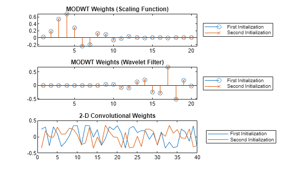
Compare the weights from the MODWT and 2-D convolutional layers along the two initialization calls. The MODWT layer sets the weights using the scaling and wavelet filters from the specified wavelet, while the convolutional layer weights consists of a new set of random values.

lgn = ["First" "Second"] + " Initialization";
weights1 = extractdata(tInit1.Value{1});
weights2 = extractdata(tInit2.Value{1});
tiledlayout vertical
nexttile
stem(weights1(1,:))
hold on
stem(weights2(1,:),"x")
hold off
title("MODWT Weights (Scaling Function)")
legend(lgn,Location="eastoutside")
nexttile
stem(weights1(2,:))
hold on
stem(weights2(2,:),"x")
hold off
title("MODWT Weights (Wavelet Filter)")
legend(lgn,Location="eastoutside")
nexttile
plot([tInit1.Value{2}(:) tInit2.Value{2}(:)])
title("2-D Convolutional Weights")
legend(lgn,Location="eastoutside")

More About

Layer Output Format

modwtLayer formats the output as "SCBT", a sequence of 1-D images where the image height corresponds to the level of the wavelet transform, the second dimension corresponds to the channel, the third dimension corresponds to the batch, and the fourth dimension corresponds to time. The kth row, where k ≤ Level, contains the kth level detail of the signal. The (Level+1)th row contains the Levelth level smooth of the signal.

• You can feed the output of modwtLayer unchanged to a 1-D convolutional layer when you want to convolve along the level ("S") dimension. For more information, see convolution1dLayer (Deep Learning Toolbox).

• To feed the output of modwtLayer to a 1-D convolutional layer when you want to convolve along the time ("T") dimension, you must place a flatten layer after the modwtLayer. For more information, see flattenLayer (Deep Learning Toolbox).

• You can feed the output of modwtLayer unchanged to a 2-D convolutional layer when you want to convolve along the level ("S") and time ("T") dimensions jointly. For more information, see convolution2dLayer (Deep Learning Toolbox).

• To use modwtLayer as part of a recurrent neural network, you must place a flatten layer after the modwtLayer. For more information, see lstmLayer (Deep Learning Toolbox) and gruLayer (Deep Learning Toolbox).

• To use the output of modwtLayer with a fully connected layer as part of a classification workflow, you must reduce the time ("T") dimension of the output so that it is of size 1. To reduce the time dimension of the output, place a global pooling layer before the fully connected layer. For more information, see globalAveragePooling2dLayer (Deep Learning Toolbox) and fullyConnectedLayer (Deep Learning Toolbox).

Extended Capabilities

C/C++ Code Generation

Generate C and C++ code using MATLAB® Coder™. (since R2025a)

Usage notes and limitations:

• The input signal to the predict function must be fixed size.

• You can generate generic C/C++ code that does not depend on third-party libraries and deploy the generated code to hardware platforms.

GPU Code Generation

Generate CUDA® code for NVIDIA® GPUs using GPU Coder™. (since R2025a)

Usage notes and limitations:

• The input signal to the predict function must be fixed size.

• You can generate CUDA code that is independent of deep learning libraries and deploy the generated code to platforms that use NVIDIA^® GPU processors.

Version History

Introduced in R2022b

R2025a: Initialize layer weights through dlnetwork initialization

Starting in R2025a, you can use initialize (Deep Learning Toolbox) to initialize learnable parameters for deep learning neural networks that include modwtLayer objects.

R2025a: New Weights default value

Starting in R2025a, the default value of the Weights property is []. Prior to R2025a, modwtLayer set the default value to the wavelet filters used in the MODWT.

R2025a: C/C++ and GPU Code Generation

The modwtLayer object supports:

• C/C++ code generation. You must have MATLAB^® Coder™ to generate C/C++ code.

• Code generation for NVIDIA GPUs. You must have GPU Coder™ to generate GPU code.