littlewoodPaleySum

Littlewood-Paley sum for JTFS filters

Since R2024b

Syntax

[lpsum1,lpsum2] = littlewoodPaleySum(jtfn)

[lpsum1,lpsum2] = littlewoodPaleySum(jtfn,FilterBank=filterbanktype)

Description

[lpsum1,lpsum2] = littlewoodPaleySum(jtfn) returns the Littlewood-Paley sums for the first- and second-order wavelet time filter banks, lpsum1 and lpsum2 respectively, in the joint time-frequency scattering (JTFS) network, jtfn.

For more information about the Littlewood-Paley sums, see Proposition 2.1 in [1].

[lpsum1,lpsum2] = littlewoodPaleySum(jtfn,FilterBank=filterbanktype) returns the Littlewood-Paley sums for the filterbanktype filter banks.

Examples

Littlewood-Paley Sums of JTFS Network

Use timeFrequencyScattering with default settings to create a joint time-frequency scattering (JTFS) network.

jtfn = timeFrequencyScattering;

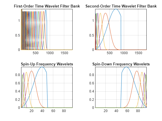
Plot the wavelet filters in the first- and second-order time filter banks, and the spin-up and spin-down wavelet filters. The filter magnitudes are not equal because, by default, the network attempts to approximate the Littlewood-Paley condition for the filters. You can change this default behavior through the EnergyCorrectFilters network property.

[psi1f,psi2f,~] = filterbank(jtfn);
[psiffrup,psiffrdn,~] = filterbank(jtfn,FilterBank="frequency");
tiledlayout(2,2)
nexttile
plot(psi1f)
grid on
axis tight
title("First-Order Time Wavelet Filter Bank")
nexttile
plot(psi2f)
grid on
axis tight
title("Second-Order Time Wavelet Filter Bank")
nexttile
plot(psiffrup)
grid on
title("Spin-Up Frequency Wavelets")
axis tight
nexttile
plot(psiffrdn)
title("Spin-Down Frequency Wavelets")
grid on
axis tight

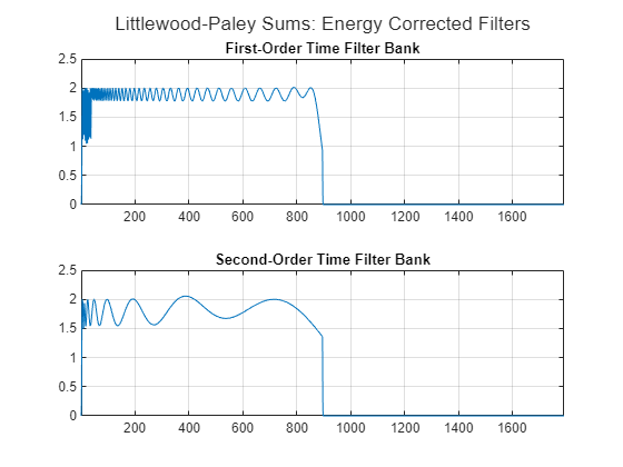
To see the effect of the approximation, use littlewoodPaleySum to plot the Littlewood-Paley sums of the first- and second-order time filter banks. In the theoretical best-case scenario, the Littlewood-Paley sum for these filters is a straight line equal to 2 from 0 to the Nyquist, and zero after that. Given the freedom you have in constructing the network, the best-case scenario is not possible. Therefore, the network approximates the filters so that the Littlewood-Paley sums are as close to 2 as possible.

[lpsum1,lpsum2] = littlewoodPaleySum(jtfn,FilterBank="time");
figure
t = tiledlayout(2,1);
nexttile
plot(lpsum1)
title("First-Order Time Filter Bank")
grid on
xlim([1 numel(lpsum1)])
nexttile
plot(lpsum2)
title("Second-Order Time Filter Bank")
xlim([1 numel(lpsum2)])
grid on
title(t,"Littlewood-Paley Sums: Energy Corrected Filters")

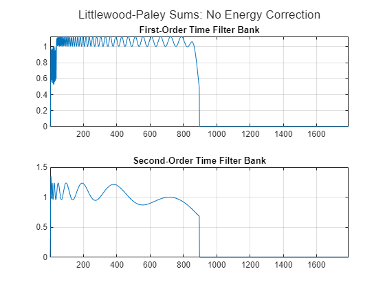
To see the impact of the energy correction, create a JTFS network with EnergyCorrectFilters set to false. Plot the Littlewood-Paley sums of the wavelet time filter banks. These sums are very different from the sums of the energy-corrected filters and far below the expected theoretical value of 2.

jtfn = timeFrequencyScattering(EnergyCorrectFilters=false);
[lpsum1,lpsum2] = littlewoodPaleySum(jtfn,FilterBank="time");
figure
t = tiledlayout(2,1);
nexttile
plot(lpsum1)
title("First-Order Time Filter Bank")
grid on
xlim([1 numel(lpsum1)])
nexttile
plot(lpsum2)
title("Second-Order Time Filter Bank")
xlim([1 numel(lpsum2)])
grid on
title(t,"Littlewood-Paley Sums: No Energy Correction")

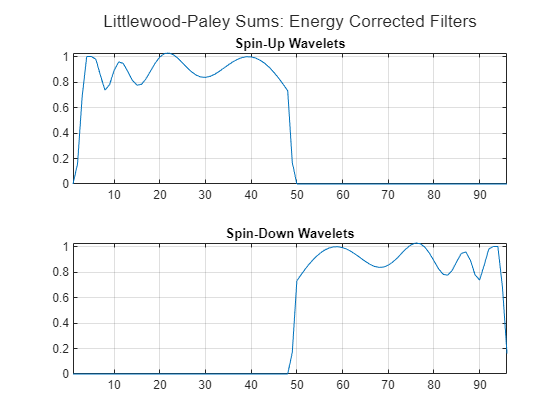
Repeat the same steps for the spin-up and spin-down wavelet filters. In the theoretical best-case scenario, the Littlewood-Paley sum for these filters would be a straight line equal to 1 across the entire range. As is the case for the time wavelet filters, it is not possible to achieve this theoretical value exactly.

Plot the Littlewood-Paley sums of the spin-up and spin-down wavelets in the default JTFS network.

jtfn = timeFrequencyScattering;
[lpsum1,lpsum2] = littlewoodPaleySum(jtfn,FilterBank="frequency");
figure
t = tiledlayout(2,1);
nexttile
plot(lpsum1)
title("Spin-Up Wavelets")
grid on
xlim([1 numel(lpsum1)])
nexttile
plot(lpsum2)
title("Spin-Down Wavelets")
xlim([1 numel(lpsum2)])
grid on
title(t,"Littlewood-Paley Sums: Energy Corrected Filters")

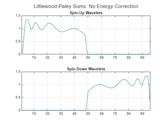
Compare with a plot of the Littlewood-Paley sums using a JTFS network with EnergyCorrectFilters set to false. Without energy correction, the sums oscillate significantly above and below the expected theoretical value of 1. The sums of the spin-up and spin-down wavelets also exhibit downward and upward trends, respectively. This behavior does not occur for the energy-corrected filters.

jtfn = timeFrequencyScattering(EnergyCorrectFilters=false);
[lpsum1,lpsum2] = littlewoodPaleySum(jtfn,FilterBank="frequency");
figure
t = tiledlayout(2,1);
nexttile
plot(lpsum1)
title("Spin-Up Wavelets")
grid on
xlim([1 numel(lpsum1)])
nexttile
plot(lpsum2)
title("Spin-Down Wavelets")
xlim([1 numel(lpsum2)])
grid on
title(t,"Littlewood-Paley Sums: No Energy Correction")

Input Arguments

jtfn — Joint time-frequency scattering network

timeFrequencyScattering object

Joint time-frequency scattering network, specified as a timeFrequencyScattering object.

filterbanktype — Filter banks type

"time" (default) | "frequency"

Filter banks type, specified as one of the following:

• "time" — First- and second-order wavelet time filter banks

• "frequency" — Spin-up and spin-down wavelet filters

Output Arguments

lpsum1 — Littlewood-Paley sum

vector

Littlewood-Paley sum of the first filterbanktype filter bank. If filterbanktype is "time", the sum is of the first-order wavelet time filter bank. If filterbanktype is "frequency", the sum is of the spin-up wavelet filters.

lpsum2 — Littlewood-Paley sum

vector

Littlewood-Paley sum of the second filterbanktype filter bank. If filterbanktype is "time", the sum is of the second-order wavelet time filter bank. If filterbanktype is "frequency", the sum is of the spin-down wavelet filters.

References

[1] Mallat, Stéphane. “Group Invariant Scattering.” Communications on Pure and Applied Mathematics 65, no. 10 (October 2012): 1331–98. https://doi.org/10.1002/cpa.21413

Version History

Introduced in R2024b