ans =
Contenuto principale
Results for
初カキコ…ども… 俺みたいな中年で深夜にMATLAB見てる腐れ野郎、 他に、いますかっていねーか、はは
今日のSNSの会話 あの流行りの曲かっこいい とか あの 服ほしい とか ま、それが普通ですわな
かたや俺は電子の砂漠でfor文無くして、呟くんすわ
it'a true wolrd.狂ってる?それ、誉め 言葉ね。
好きなtoolbox Signal Processing Toolbox
尊敬する人間 Answersの海外ニキ(学校の課題質問はNO)
なんつってる間に4時っすよ(笑) あ~あ、休日の辛いとこね、これ
-----------
ディスカッションに記事を書いたら謎の力によって消えたっぽいので、性懲りもなくだらだら書いていこうと思います。前書いた内容忘れたからテキトーに書きます。
救いたいんですよ、Centralを(倒置法)
いっぬはMATLAB Answersに育てられてキャリアを積んできたんですよ。暇な時間を見つけてはAnswersで回答して承認欲求を満たしてきたんです。わかんない質問に対しては別の人が回答したのを学び、応用してバッジもらったりしちゃったりしてね。
そんな思い出の大事な1ピースを担うMATLAB Centralが、いま、苦境に立たされている。僕はMATLAB Centralを救いたい。
最悪、救うことが出来なくともCentralと一緒に死にたい。Centralがコミュニティを閉じるのに合わせて、僕の人生の幕も閉じたい。MATLABメンヘラと呼ばれても構わない。MATLABメンヘラこそ、MATLABに対する愛の証なのだ。MATLABメンヘラと呼ばれても、僕は強く生きる。むしろ、誇りに思うだろう。
こうしてMATLABメンヘラへの思いの丈を精一杯綴った今、僕はこう思う。
MATLABメンヘラって何?
なぜ苦境に立っているのか?
生成AIである。Hernia Babyは激怒した。必ず、かの「もうこれでいいじゃん」の王を除かなければならぬと決意した。Hernia BabyにはAIの仕組みがわからぬ。Hernia Babyは、会社の犬畜生である。マネージャが笛を吹き、エナドリと遊んで暮して来た。けれどもネットmemeに対しては、人一倍に敏感であった。
風の噂によるとMATLAB Answersの質問数も微妙に減少傾向にあるそうな。
確かにTwitter(現X)でもAnswers botの呟き減ったような…。
ゆ、許せんぞ生成AI…!
MATLAB Centralは日本では流行ってない?
そもそもCentralって日本じゃあまりアクセスされてないんじゃなイカ?
だってどうやってここにたどり着けばいいかわかんねえもん!(暴言)
MATLABのHPにはないから一回コミュニティのプロファイル入って…
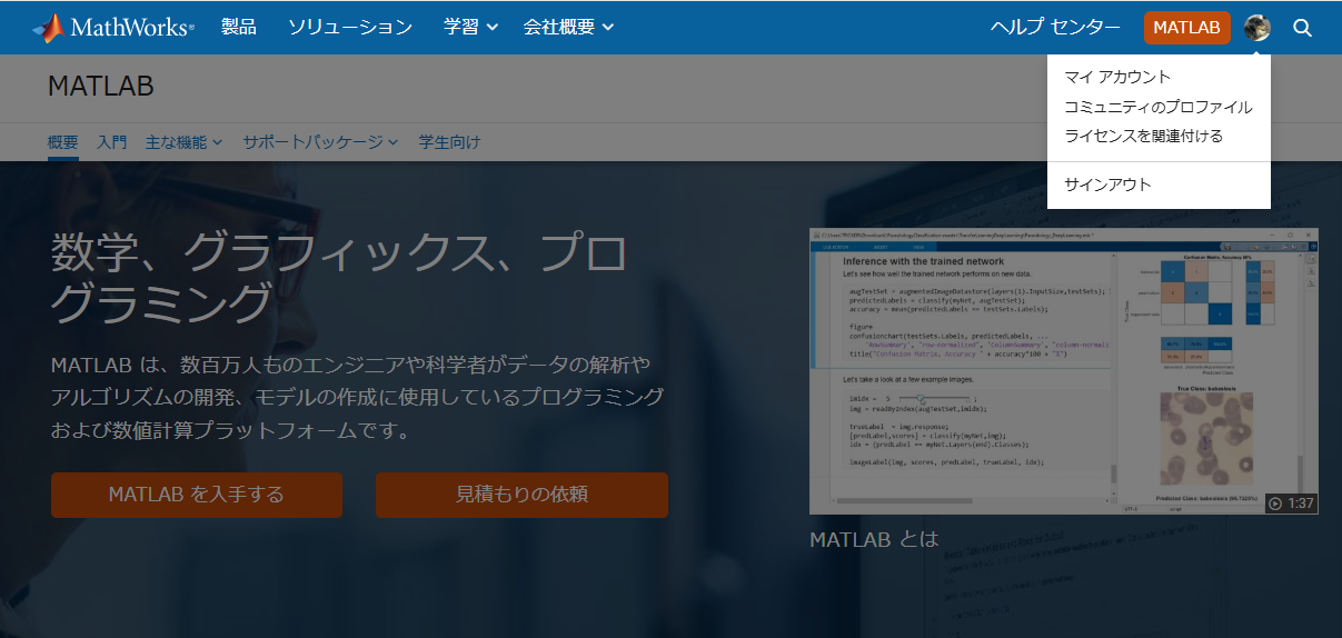
やっと表示される。気づかんって!

MATLAB Centralは無料で学べる宝物庫
とはいえ本当にオススメなんです。
どんなのがあるかさらっと紹介していきます。
ここは短い文章で問題を解くコードを書き上げるところ。
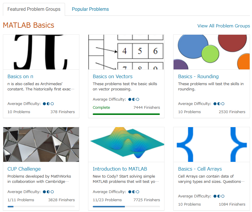
多様な分野を実践的に学ぶことができるし、何より他人のコードも見ることができる。
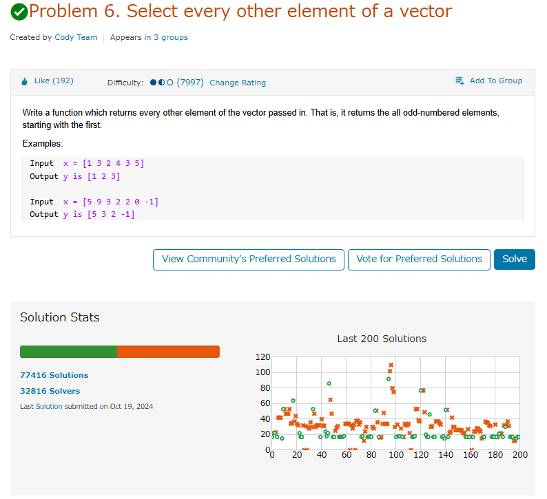
たまにそんなのありかよ~って回答もあるけどいい訓練になる。
ただ英語の問題見たらさ~ 悪い やっぱつれぇわ…
我らがアイドルmichioニキやJiro氏が新機能について紹介なんかもしてくれてる。
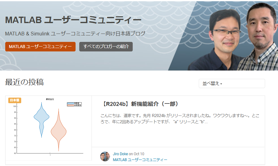
なんだかんだTwitter(現X)で紹介しちゃってるから、見るのさぼったり…ゲフンゲフン!
定期的に開催される。
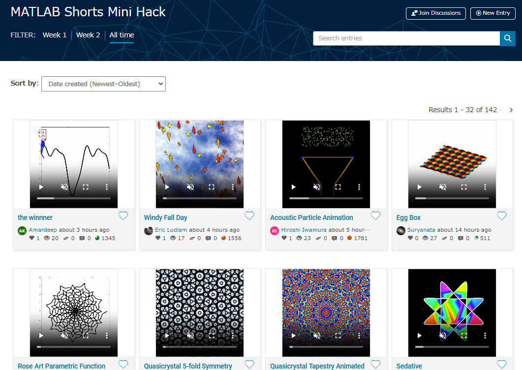
プライズも貰えたりするし、何よりめっちゃ面白い作品を皆が書いてくる。
p=pi;
l = 5e3;
m = 0:l;
[u,v]=meshgrid(10*m/l*p,2*m/l*p);
c=cos(v/2);
s=sin(v);
e=1-exp(u/(6*p));
surf(2*e.*cos(u).*c.^2,-e*2.*sin(u).*c.^2,1-exp(u/(3.75*p))-s+exp(u/(5.5*p)).*s,'FaceColor','#a47a43','EdgeAlpha',0.02)
axis equal off
A=7.3;
zlim([-A 0])
view([-12 23])
set(gcf,'Color','#d2b071')
過去の事は水に流してくれないか?
toolboxにない自作関数とかを無料で皆が公開してるところ。
MATLABのアドオンからだと関数をそのままインストール出来たりする。
だいたいの答えはここにある。質問する前にググれば出てくる。
躓いて調べると過去に書いてあった自分の回答に助けられたりもする。
for文で回答すると一定数の海外ニキたちが
と絡んでくる。
Answersがバキバキ回答する場であるのに対して、ここでは好きなことを呟いていいらしい。最近できたっぽい。全然知らんかった。海外では「こんな機能欲しくね?」とかけっこう人気っぽい。
日本人が書いてないから僕がこんなクソスレ書いてるわけ┐(´д`)┌ヤレヤレ
まとめ
いかがだったでしょうか?このようにCentralは学びとして非常に有効な場所なのであります。インプットもいいけど是非アウトプットしてみましょう。コミュニティはアカウントさえ持ってたら無料でやれるんでね。
皆はどうやってMATLAB/Simulinkを学んだか、良ければ返信でクソレスしてくれると嬉しいです。特にSimulinkはマジでな~んにもわからん。MathWorksさんode45とかソルバーの説明ここでしてくれ。
後、ディスカッション一時保存機能つけてほしい。
最後に
Centralより先に、俺を救え
参考:ミスタードーナツを救え
Here presented MATLAB code is designed to create a seamless loop animation that visualizes an isosurface derived from random data.
This entry, titled "The Scrambled Predator's Cube", builds upon my previous work and has been adapted to include dynamic elements.
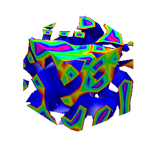
In this explanation, I will break down the relatively short code, making it accessible whether you are a beginner in MATLAB or an experienced user. Let's go through the MATLAB code step by step to understand each line in detail.
Code Breakdown
d = rand(8,8,8);
Random Data Generation: This line creates a three-dimensional array d with dimensions 8×8×8 filled with random values. The rand function generates values uniformly distributed in the interval (0,1). This array serves as the input data for generating the isosurface.
iv = .5 + (f / 10000);
Isovalue Calculation: Here, the isovalue iv is computed based on the frame number f. The expression f / 10000 causes iv to increase very slowly as f increments. Starting from 0.50, this means that for every increment of f, iv changes slightly (specifically, by 0.0001). This gradual increase creates a smooth transition effect in the isosurface over time, making it look dynamic as the animation progresses.
h = patch(isosurface(d, iv), 'FaceColor', 'blue', 'EdgeColor', 'none');
Isosurface Creation: The isosurface function extracts a 3D surface from the data array d at the specified isovalue iv. The result is a patch object h that represents the isosurface in the 3D plot. The 'FaceColor', 'blue' argument sets the face color of the surface to blue, while 'EdgeColor', 'none' specifies that no edges should be drawn, giving the surface a solid appearance.
isonormals(d, h);
Surface Normals Calculation: This function calculates the normals at each vertex of the isosurface h, based on the data in d. Normals are vectors perpendicular to the surface at each point and are crucial for proper lighting calculations. By using isonormals, the appearance of depth and texture is enhanced, allowing the lighting to interact more realistically with the surface.
patch(isocaps(d, iv), 'FaceColor', 'interp', 'EdgeColor', 'none');
Isocaps Visualization: The isocaps function creates flat surfaces (caps) at the boundaries of the isosurface where the data values meet the isovalue iv. The resulting caps are then rendered as patches with 'FaceColor', 'interp', meaning the colors of the caps are interpolated based on the data values. The caps provide a more complete visual representation of the isosurface, improving its overall appearance.
colormap hsv;
Color Map Setup: This line sets the colormap of the current figure to HSV (Hue, Saturation, Value). The HSV colormap allows for a wide range of colors, which can enhance the visual appeal of the rendering by mapping different values in the data to different colors.
daspect([1, 1, 1]);
Aspect Ratio Setting: The daspect function sets the data aspect ratio of the plot to be equal in all three dimensions. This means that one unit in the x-direction is the same length as one unit in the y-direction and z-direction, ensuring that the visual representation of the 3D data is not distorted.
axis tight;
Tight Axis Setting: This command adjusts the limits of the axes so that they fit tightly around the data, removing any excess white space. It helps to focus the viewer's attention on the isosurface and related visual elements.
view(3);
3D View Configuration: The view(3) command sets the current view to a 3D perspective, allowing the viewer to see the structure of the isosurface from an angle that reveals its three-dimensional nature.
camlight right;
camlight left;
Lighting Effects: These commands add two light sources to the scene, positioned to the right and left of the view. The additional lighting enhances the shading and depth perception of the isosurface, making it appear more three-dimensional and visually appealing.
axis off;
Hide Axes: This command turns off the display of the axes in the plot. Removing the axes provides a cleaner visual representation, allowing the viewer to focus solely on the isosurface and its lighting effects without distraction from the grid lines or axis labels.
lighting phong;
Lighting Model: This line sets the lighting model to Phong. The Phong model is widely used in computer graphics as it provides smooth shading and realistic reflections. It calculates how light interacts with surfaces, enhancing the overall appearance by creating a more natural look.
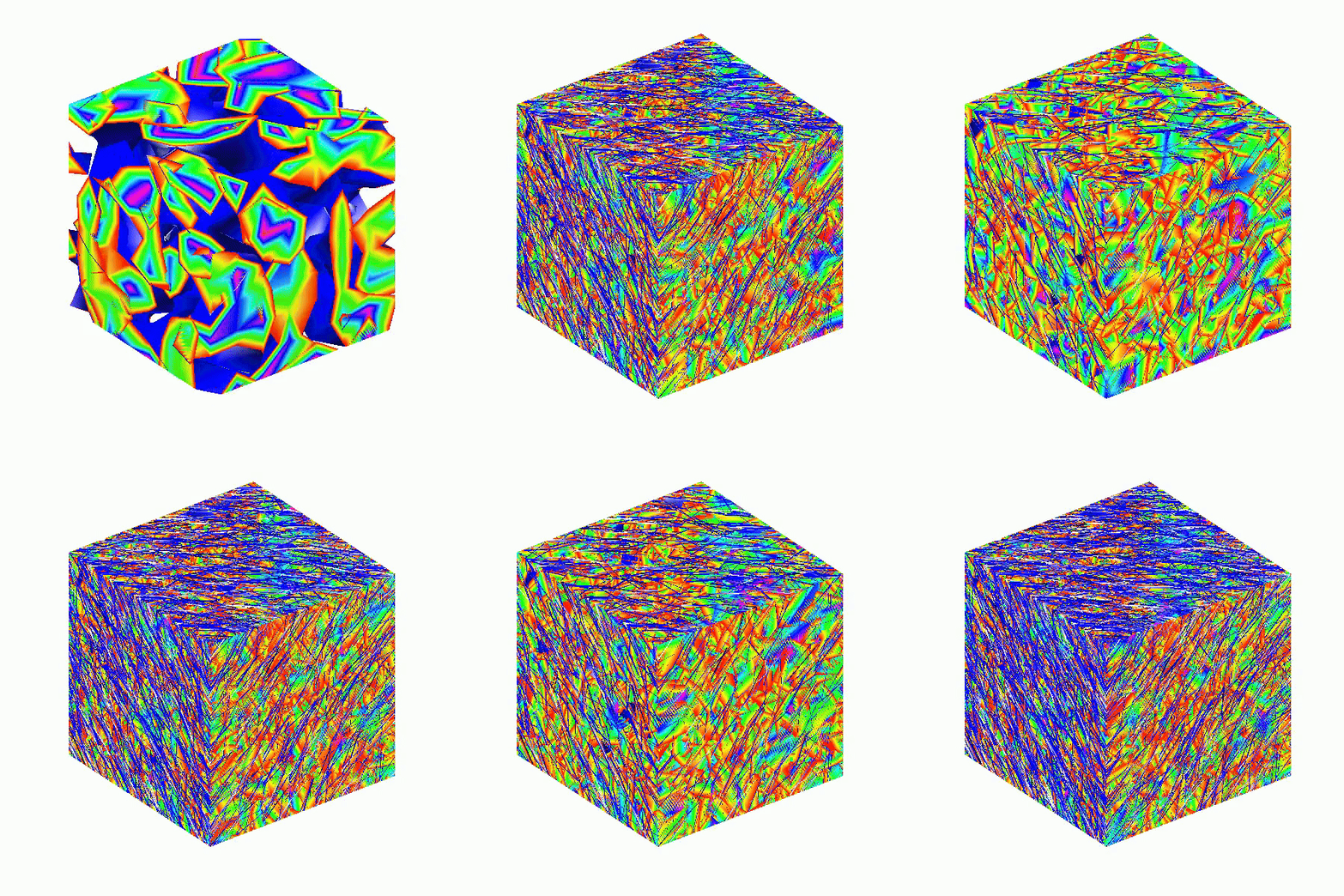
This code creates a visually dynamic and appealing representation of an isosurface derived from random data. The gradual change in the isovalue allows for smooth transitions, while the combination of lighting, colors, and shading contributes to a rich 3D visualization. Each component plays a vital role in rendering the final output, showcasing advanced techniques in data visualization using MATLAB.
I'd like to share some tips about the 2024 mini hack contest, specifically related to audio:
- First (and most important), credit your source: unless you are composing your own audio, I think it's important to give credit to the original sources. It is a little sad to see several contributions with an empty line:
'Cite your audio source here (if applicable):'
- A great place to get royalty-free and high-quality music and audio (among other media) is https://pixabay.com. Be sure to check it out! I used one of their audio clips in my submission EKG pulse
- The right music can enhance the overall experience of your animation. Sometimes getting the animation to match the music beat can be hard. I suggest you try the other way around: get your music/sound effects to match the animation rhythm with a little editing. A free audio editor with many capabilities (more than enough for this contest, I think) is https://www.audacityteam.org/
- Choose a 4-second audio clip with a consistent tempo and seamless loop points, ensuring it complements your animation's mood and loops smoothly over 12 seconds without abrupt changes.
I think that when the right music is paired with the right animation, it can create a more impactful experience.
Well, this is my first time to participate in such community competitions and guess what, I've gone for 4 submissions so far (Feels Great!!)
So I wanna share some tricks that I followed for my first submission named Happy Shaping' ( Go Check it out!!):
1. Dynamic Background Color Change:
- Technique: The background color of the figure window is gradually changed using sine and cosine functions.
- Reason: These trigonometric functions (sin and cos) create smooth, oscillating transitions over time, which gives a fluid effect to the background's color shift.
- Implementation:
Color = [0.1 + 0.5*abs(sin(f/10)), 0.1 + 0.5*abs(cos(f/15)), 0.9 -
0.5*abs(sin(f/20))];
- Benefit: This introduces a smooth, visually appealing animation effect.
2. Smooth Object Motion Using Sine and Cosine:
- Technique: The position and shape of objects are based on trigonometric functions.
- Reason: Using sin(t) and cos(t) ensures that the movement is circular or elliptical, creating continuous and natural motion in animations.
- Implementation (for object position):
x = 10 * cos(t * 2 * pi) * (1 + 0.5 * sin(t * pi));
y = 10 * sin(t * 2 * pi) * (1 + 0.5 * cos(t * pi));
- Benefit: Circular and smooth motions are pleasing and easily controlled by tweaking the frequency and phase of sine/cosine functions.
3. Polygon Shape Changing Over Time:
- Technique: The number of sides of the polygon (sides) changes dynamically based on t.
- Reason: It creates variation in shape, maintaining user interest as the shape transitions from a triangle to a hexagon.
- Implementation:
sides = 3 + round(3 * abs(sin(t)));
- Benefit: This provides dynamic shape transitions over time, keeping the animation non-static.
4. Use of the fill Function for Color-Filled Shapes:
- Technique: The fill function is used to draw a polygon with smoothly changing colors.
- Reason: Filling polygons with varying colors based on time (t) allows for continuous color transitions, adding more complexity to the animation.
- Implementation:
fill(xp, yp, c, 'EdgeColor', 'none');
- Benefit: Combining both color changes and shape changes enhances the visual impact.
5. Consistent Use of hold on and hold off:
- Technique: hold on allows multiple graphic objects to be drawn on the same axes without clearing previous objects.
- Reason: This is crucial for drawing multiple elements (like polygons, circles, and lines) on the same figure.
- Benefit: It helps manage and layer different graphical elements effectively within the same frame.
6. Use of rectangle for a Smooth Ball Motion:
- Technique: The ball's motion is defined by rectangle with a Curvature of [1, 1] to make it circular.
- Reason: Using the rectangle function simplifies the process of drawing a filled circle, and controlling its position and size is intuitive.
- Benefit: It provides a straightforward way to animate circular objects within the plot.
7. Animating the Connection Line:
- Technique: A white dashed line (w--) is drawn between the polygon and the moving ball to show a connection between these objects.
- Reason: This adds interactivity to the scene, as it gives the impression that the polygon and the ball are related or connected in some way.
- Implementation:
plot([x bx], [y by], 'w--', 'LineWidth', 2);
- Benefit: A dynamic element that adds depth and narrative to the animation, guiding the viewer’s attention.
8. Frame Synchronization with Time (f and t):
- Technique: The variable f is used as a frame number, while t = f / 24 creates a link between frame and time.
- Reason: Ensuring smooth and continuous transitions in the animation over time is critical, so f acts as the control for time-based changes in shape, color, and position.
- Benefit: This makes it easy to manage frame rates and time-based updates for the animation.
If you like them, please feel free to use them for free.
Let's say you have a chance to ask the MATLAB leadership team any question. What would you ask them?
hello i found the following tools helpful to write matlab programs. copilot.microsoft.com chatgpt.com/gpts gemini.google.com and ai.meta.com. thanks a lot and best wishes.
If I go to a paint store, I can get foldout color charts/swatches for every brand of paint. I can make a selection and it will tell me the exact proportions of each of base color to add to a can of white paint. There doesn't seem to be any equivalent in MATLAB. The common word "swatch" doesn't even exist in the documentation. (?) One thinks pcolor() would be the way to go about this, but pcolor documentation is the most abstruse in all of the documentation. Thanks 1e+06 !
What is the side-effect of counting the number of Deep Learning Toolbox™ updates in the last 5 years? The industry has slowly stabilised and matured, so updates have slowed down in the last 1 year, and there has been no exponential growth.Is it correct to assume that? Let's see what you think!
releaseNumNames = "R"+string(2019:2024)+["a";"b"];
releaseNumNames = releaseNumNames(:);
numReleaseNotes = [10,14,27,39,38,43,53,52,55,57,46,46];
exampleNums = [nan,nan,nan,nan,nan,nan,40,24,22,31,24,38];
bar(releaseNumNames,[numReleaseNotes;exampleNums]')
legend(["#release notes","#new/update examples"],Location="northwest")
title("Number of Deep Learning Toolbox™ update items in the last 5 years")
ylabel("#release notes")
As pointed out in Doxygen comments in code generated with Simulink Embedded Coder - MATLAB Answers - MATLAB Central (mathworks.com), it would be nice that Embedded Coder has an option to generate Doxygen-style comments for signals of buses, i.e.:
/** @brief <Signal desciption here> **/
This would allow static analysis tools to parse the comments. Please add that feature!

See the attached PDF for a higher resolution
Related blogs posts:
Local large language models (LLMs), such as llama, phi3, and mistral, are now available in the Large Language Models (LLMs) with MATLAB repository through Ollama™!
Read about it here:
Hot off the heels of my High Performance Computing experience in the Czech republic, I've just booked my flights to Atlanta for this year's supercomputing conference at SC24.
Will any of you be there?
syms u v
atan2alt(v,u)
function Z = atan2alt(V,U)
% extension of atan2(V,U) into the complex plane
Z = -1i*log((U+1i*V)./sqrt(U.^2+V.^2));
% check for purely real input. if so, zero out the imaginary part.
realInputs = (imag(U) == 0) & (imag(V) == 0);
Z(realInputs) = real(Z(realInputs));
end
As I am editing this post, I see the expected symbolic display in the nice form as have grown to love. However, when I save the post, it does not display. (In fact, it shows up here in the discussions post.) This seems to be a new problem, as I have not seen that failure mode in the past.
You can see the problem in this Answer forum response of mine, where it did fail.
In case you haven't come across it yet, @Gareth created a Jokes toolbox to get MATLAB to tell you a joke.
As far as I know, starting from MATLAB R2024b, the documentation is defaulted to be accessed online. However, the problem is that every time I open the official online documentation through my browser, it defaults or forcibly redirects to the documentation hosted site for my current geographic location, often with multiple pop-up reminders, which is very annoying!
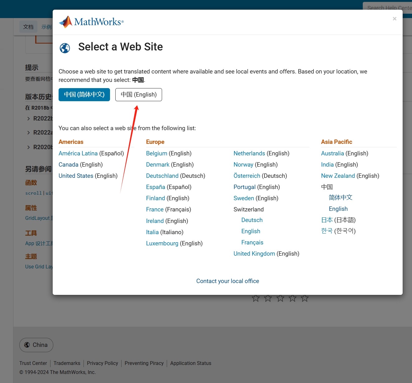
Suggestion: Could there be an option to set preferences linked to my personal account so that the documentation defaults to my chosen language preference without having to deal with “forced reminders” or “forced redirection” based on my geographic location? I prefer reading the English documentation, but the website automatically redirects me to the Chinese documentation due to my geolocation, which is quite frustrating!
----------------2024.12.13 update-----------------
Although the above issue was resolved by technical support, subsequent redirects are still causing severe delays...
In the past two years, MATHWORKS has updated the image viewer and audio viewer, giving them a more modern interface with features like play, pause, fast forward, and some interactive tools that are more commonly found in typical third-party players. However, the video player has not seen any updates. For instance, the Video Viewer or vision.VideoPlayer could benefit from a more modern player interface. Perhaps I haven't found a suitable built-in player yet. It would be great if there were support for custom image processing and audio processing algorithms that could be played in a more modern interface in real time.
Additionally, I found it quite challenging to develop a modern video player from scratch in App Designer.(If there's a video component for that that would be great)
-----------------------------------------------------------------------------------------------------------------
BTW,the following picture shows the built-in function uihtml function showing a more modern playback interface with controls for play, pause and so on. But can not add real-time image processing algorithms within it.

I was browsing the MathWorks website and decided to check the Cody leaderboard. To my surprise, William has now solved 5,000 problems. At the moment, there are 5,227 problems on Cody, so William has solved over 95%. The next competitor is over 500 problems behind. His score is also clearly the highest, approaching 60,000.
Has this been eliminated? I've been at 31 or 32 for 30 days for awhile, but no badge. 10 badge was automatic.


