Risultati per
I’m currently developing a multi-platform viewer using Flutter to eliminate the hassle of manual channel setup. Instead of adding IDs one by one, the app uses your User API Key to automatically discover and list all your ThingSpeak channels instantly.
Key Highlights (Work in Progress):
- Automatic Sync: All your channels appear in seconds.
- Multi-platform: Built for Web, Android, Windows, and Linux.
- Privacy-Focused: Secure local storage for your API keys.
If you use tables extensively to perform data analysis, you may at some point have wanted to add new functionalities suited to your specific applications. One straightforward idea is to create a new class that subclasses the built-in table class. You would then benefit from all inherited existing methods.
One workaround is to create a new class that wraps a table as a Property, and re-implement all the methods that you need and are already defined for table. The is not too difficult, except for the subsref method, for which I’ll provide the code below.
Class definition
Defining a wrapper of the table class is quite straightforward. In this example, I call the class “Report” because that is what I intend to use the class for, to compute and store reports. The constructor just takes a table as input:
classdef Rapport
methods
function obj = Report(t)
if isa(t, 'Report')
obj = t;
else
obj.t_ = t;
end
end
end
properties (GetAccess = private, SetAccess = private)
t_ table = table();
end
end
I designed the constructor so that it converts a table into a Report object, but also so that if we accidentally provide it with a Report object instead of a table, it will not generate an error.
Reproducing the behaviour of the table class
Implementing the existing methods of the table class for the Report class if pretty easy in most cases.
I made use of a method called “table” in order to be able to get the data back in table format instead of a Report, instead of accessing the property t_ of the object. That method can also be useful whenever you wish to use the methods or functions already existing for tables (such as writetable, rowfun, groupsummary…).
classdef Rapport
...
methods
function t = table(obj)
t = obj.t_;
end
function r = eq(obj1,obj2)
r = isequaln(table(obj1), table(obj2));
end
function ind = size(obj, varargin)
ind = size(table(obj), varargin{:});
end
function ind = height(obj, varargin)
ind = height(table(obj), varargin{:});
end
function ind = width(obj, varargin)
ind = width(table(obj), varargin{:});
end
function ind = end(A,k,n)
% ind = end(A.t_,k,n);
sz = size(table(A));
if k < n
ind = sz(k);
else
ind = prod(sz(k:end));
end
end
end
end
In the case of horzcat (same principle for vertcat), it is just a matter of converting back and forth between the table and Report classes:
classdef Rapport
...
methods
function r = horzcat(obj1,varargin)
listT = cell(1, nargin);
listT{1} = table(obj1);
for k = 1:numel(varargin)
kth = varargin{k};
if isa(kth, 'Report')
listT{k+1} = table(kth);
elseif isa(kth, 'table')
listT{k+1} = kth;
else
error('Input must be a table or a Report');
end
end
res = horzcat(listT{:});
r = Report(res);
end
end
end
Adding a new method
The plus operator already exists for the table class and works when the table contains all numeric values. It sums columns as long as the tables have the same length.
Something I think would be nice would be to be able to write t1 + t2, and that would perform an outerjoin operation between the tables and any sizes having similar indexing columns.
That would be so concise, and that's what we’re going to implement for the Report class as an example. That is called “plus operator overloading”. Of course, you could imagine that the “+” operator is used to compute something else, for example adding columns together with regard to the keys index. That depends on your needs.
Here’s a unittest example:
classdef ReportTest < matlab.unittest.TestCase
methods (Test)
function testPlusOperatorOverload(testCase)
t1 = array2table( ...
{ 'Smith', 'Male' ...
; 'JACKSON', 'Male' ...
; 'Williams', 'Female' ...
} , 'VariableNames', {'LastName' 'Gender'} ...
);
t2 = array2table( ...
{ 'Smith', 13 ...
; 'Williams', 6 ...
; 'JACKSON', 4 ...
}, 'VariableNames', {'LastName' 'Age'} ...
);
r1 = Report(t1);
r2 = Report(t2);
tRes = r1 + r2;
tExpected = Report( array2table( ...
{ 'JACKSON' , 'Male', 4 ...
; 'Smith' , 'Male', 13 ...
; 'Williams', 'Female', 6 ...
} , 'VariableNames', {'LastName' 'Gender' 'Age'} ...
) );
testCase.verifyEqual(tRes, tExpected);
end
end
end
And here’s how I’d implement the plus operator in the Report class definition, so that it also works if I add a table and a Report:
classdef Rapport
...
methods
function r = plus(obj1,obj2)
table1 = table(obj1);
table2 = table(obj2);
result = outerjoin(table1, table2 ...
, 'Type', 'full', 'MergeKeys', true);
r = reportingits.dom.Rapport(result);
end
end
end
The case of the subsref method
If we wish to access the elements of an instance the same way we would with regular tables, whether with parentheses, curly braces or directly with the name of the column, we need to implement the subsref and subsasgn methods. The second one, subsasgn is pretty easy, but subsref is a bit tricky, because we need to detect whether we’re directing towards existing methods or not.
Here’s the code:
classdef Rapport
...
methods
function A = subsasgn(A,S,B)
A.t_ = subsasgn(A.t_,S,B);
end
function B = subsref(A,S)
isTableMethod = @(m) ismember(m, methods('table'));
isReportMethod = @(m) ismember(m, methods('Report'));
switch true
case strcmp(S(1).type, '.') && isReportMethod(S(1).subs)
methodName = S(1).subs;
B = A.(methodName)(S(2).subs{:});
if numel(S) > 2
B = subsref(B, S(3:end));
end
case strcmp(S(1).type, '.') && isTableMethod (S(1).subs)
methodName = S(1).subs;
if ~isReportMethod(methodName)
error('The method "%s" needs to be implemented!', methodName)
end
otherwise
B = subsref(table(A),S(1));
if istable(B)
B = Report(B);
end
if numel(S) > 1
B = subsref(B, S(2:end));
end
end
end
end
end
Conclusion
I believe that the table class is Sealed because is case new methods are introduced in MATLAB in the future, the subclass might not be compatible if we created any or generate unexpected complexity.
The table class is a really powerful feature.
I hope this example has shown you how it is possible to extend the use of tables by adding new functionalities and maybe given you some ideas to simplify some usages. I’ve only happened to find it useful in very restricted cases, but was still happy to be able to do so.
In case you need to add other methods of the table class, you can see the list simply by calling methods(’table’).
Feel free to share your thoughts or any questions you might have! Maybe you’ll decide that doing so is a bad idea in the end and opt for another solution.
Give your LLM an easier time looking for information on mathworks.com: point it to the recently released llms.txt files. The top-level one is www.mathworks.com/llms.txt, release changes use www.mathworks.com/help/relnotes. How does it work for you??
I can't believe someone put time into this ;-)

Our exportgraphics and copygraphics functions now offer direct and intuitive control over the size, padding, and aspect ratio of your exported figures.
- Specify Output Size: Use the new Width, Height, and Units name-value pairs
- Control Padding: Easily adjust the space around your axes using the Padding argument, or set it to to match the onscreen appearance.
- Preserve Aspect Ratio: Use PreserveAspectRatio='on' to maintain the original plot proportions when specifying a fixed size.
- SVG Export: The exportgraphics function now supports exporting to the SVG file format.
Check out the full article on the Graphics and App Building blog for examples and details: Advanced Control of Size and Layout of Exported Graphics
No, staying home (or where I'm now)
25%
Yes, 1 night
0%
Yes, 2 nights
12.5%
Yes, 3 nights
12.5%
Yes, 4-7 nights
25%
Yes, 8 nights or more
25%
8 voti
Hi everyone
I've been using ThingSpeak for several years now without an issue until last Thursday.
I have four ThingSpeak channels which are used by three Arduino devices (in two locations/on two distinct networks) all running the same code.
All three devices stopped being able to write data to my ThingSpeak channels around 17:00 CET on 4 Dec and are still unable to.
Nothing changed on this side, let alone something that would explain the problem.
I would note that data can still be written to all the channels via a browser so there is no fundamental problem with the channels (such as being full).
Since the above date and time, any HTTP/1.1 'update' (write) requests via the REST API (using both simple one-write GET requests or bulk JSON POST requests) are timing out after 5 seconds and no data is being written. The 5 second timeout is my Arduino code's default, but even increasing it to 30 seconds makes no difference. Before all this, responses from ThingSpeak were sub-second.
I have recompiled the Arduino code using the latest libraries and that didn't help.
I have tested the same code again another random api (api.ipify.org) and that works just fine.
Curl works just fine too, also usng HTTP/1.1
So the issue appears to be something particular to the combination of my Arduino code *and* the ThingSpeak environment, where something changed on the ThingSpeak end at the above date and time.
If anyone in the community has any suggestions as to what might be going on, I would greatly appreciate the help.
Peter

The formula comes from @yuruyurau. (https://x.com/yuruyurau)
digital life 1

figure('Position',[300,50,900,900], 'Color','k');
axes(gcf, 'NextPlot','add', 'Position',[0,0,1,1], 'Color','k');
axis([0, 400, 0, 400])
SHdl = scatter([], [], 2, 'filled','o','w', 'MarkerEdgeColor','none', 'MarkerFaceAlpha',.4);
t = 0;
i = 0:2e4;
x = mod(i, 100);
y = floor(i./100);
k = x./4 - 12.5;
e = y./9 + 5;
o = vecnorm([k; e])./9;
while true
t = t + pi/90;
q = x + 99 + tan(1./k) + o.*k.*(cos(e.*9)./4 + cos(y./2)).*sin(o.*4 - t);
c = o.*e./30 - t./8;
SHdl.XData = (q.*0.7.*sin(c)) + 9.*cos(y./19 + t) + 200;
SHdl.YData = 200 + (q./2.*cos(c));
drawnow
end
digital life 2

figure('Position',[300,50,900,900], 'Color','k');
axes(gcf, 'NextPlot','add', 'Position',[0,0,1,1], 'Color','k');
axis([0, 400, 0, 400])
SHdl = scatter([], [], 2, 'filled','o','w', 'MarkerEdgeColor','none', 'MarkerFaceAlpha',.4);
t = 0;
i = 0:1e4;
x = i;
y = i./235;
e = y./8 - 13;
while true
t = t + pi/240;
k = (4 + sin(y.*2 - t).*3).*cos(x./29);
d = vecnorm([k; e]);
q = 3.*sin(k.*2) + 0.3./k + sin(y./25).*k.*(9 + 4.*sin(e.*9 - d.*3 + t.*2));
SHdl.XData = q + 30.*cos(d - t) + 200;
SHdl.YData = 620 - q.*sin(d - t) - d.*39;
drawnow
end
digital life 3

figure('Position',[300,50,900,900], 'Color','k');
axes(gcf, 'NextPlot','add', 'Position',[0,0,1,1], 'Color','k');
axis([0, 400, 0, 400])
SHdl = scatter([], [], 1, 'filled','o','w', 'MarkerEdgeColor','none', 'MarkerFaceAlpha',.4);
t = 0;
i = 0:1e4;
x = mod(i, 200);
y = i./43;
k = 5.*cos(x./14).*cos(y./30);
e = y./8 - 13;
d = (k.^2 + e.^2)./59 + 4;
a = atan2(k, e);
while true
t = t + pi/20;
q = 60 - 3.*sin(a.*e) + k.*(3 + 4./d.*sin(d.^2 - t.*2));
c = d./2 + e./99 - t./18;
SHdl.XData = q.*sin(c) + 200;
SHdl.YData = (q + d.*9).*cos(c) + 200;
drawnow; pause(1e-2)
end
digital life 4

figure('Position',[300,50,900,900], 'Color','k');
axes(gcf, 'NextPlot','add', 'Position',[0,0,1,1], 'Color','k');
axis([0, 400, 0, 400])
SHdl = scatter([], [], 1, 'filled','o','w', 'MarkerEdgeColor','none', 'MarkerFaceAlpha',.4);
t = 0;
i = 0:4e4;
x = mod(i, 200);
y = i./200;
k = x./8 - 12.5;
e = y./8 - 12.5;
o = (k.^2 + e.^2)./169;
d = .5 + 5.*cos(o);
while true
t = t + pi/120;
SHdl.XData = x + d.*k.*sin(d.*2 + o + t) + e.*cos(e + t) + 100;
SHdl.YData = y./4 - o.*135 + d.*6.*cos(d.*3 + o.*9 + t) + 275;
SHdl.CData = ((d.*sin(k).*sin(t.*4 + e)).^2).'.*[1,1,1];
drawnow;
end
digital life 5

figure('Position',[300,50,900,900], 'Color','k');
axes(gcf, 'NextPlot','add', 'Position',[0,0,1,1], 'Color','k');
axis([0, 400, 0, 400])
SHdl = scatter([], [], 1, 'filled','o','w',...
'MarkerEdgeColor','none', 'MarkerFaceAlpha',.4);
t = 0;
i = 0:1e4;
x = mod(i, 200);
y = i./55;
k = 9.*cos(x./8);
e = y./8 - 12.5;
while true
t = t + pi/120;
d = (k.^2 + e.^2)./99 + sin(t)./6 + .5;
q = 99 - e.*sin(atan2(k, e).*7)./d + k.*(3 + cos(d.^2 - t).*2);
c = d./2 + e./69 - t./16;
SHdl.XData = q.*sin(c) + 200;
SHdl.YData = (q + 19.*d).*cos(c) + 200;
drawnow;
end
digital life 6

clc; clear
figure('Position',[300,50,900,900], 'Color','k');
axes(gcf, 'NextPlot','add', 'Position',[0,0,1,1], 'Color','k');
axis([0, 400, 0, 400])
SHdl = scatter([], [], 2, 'filled','o','w', 'MarkerEdgeColor','none', 'MarkerFaceAlpha',.4);
t = 0;
i = 1:1e4;
y = i./790;
k = y; idx = y < 5;
k(idx) = 6 + sin(bitxor(floor(y(idx)), 1)).*6;
k(~idx) = 4 + cos(y(~idx));
while true
t = t + pi/90;
d = sqrt((k.*cos(i + t./4)).^2 + (y/3-13).^2);
q = y.*k.*cos(i + t./4)./5.*(2 + sin(d.*2 + y - t.*4));
c = d./3 - t./2 + mod(i, 2);
SHdl.XData = q + 90.*cos(c) + 200;
SHdl.YData = 400 - (q.*sin(c) + d.*29 - 170);
drawnow; pause(1e-2)
end
digital life 7

clc; clear
figure('Position',[300,50,900,900], 'Color','k');
axes(gcf, 'NextPlot','add', 'Position',[0,0,1,1], 'Color','k');
axis([0, 400, 0, 400])
SHdl = scatter([], [], 2, 'filled','o','w', 'MarkerEdgeColor','none', 'MarkerFaceAlpha',.4);
t = 0;
i = 1:1e4;
y = i./345;
x = y; idx = y < 11;
x(idx) = 6 + sin(bitxor(floor(x(idx)), 8))*6;
x(~idx) = x(~idx)./5 + cos(x(~idx)./2);
e = y./7 - 13;
while true
t = t + pi/120;
k = x.*cos(i - t./4);
d = sqrt(k.^2 + e.^2) + sin(e./4 + t)./2;
q = y.*k./d.*(3 + sin(d.*2 + y./2 - t.*4));
c = d./2 + 1 - t./2;
SHdl.XData = q + 60.*cos(c) + 200;
SHdl.YData = 400 - (q.*sin(c) + d.*29 - 170);
drawnow; pause(5e-3)
end
digital life 8

clc; clear
figure('Position',[300,50,900,900], 'Color','k');
axes(gcf, 'NextPlot','add', 'Position',[0,0,1,1], 'Color','k');
axis([0, 400, 0, 400])
SHdl{6} = [];
for j = 1:6
SHdl{j} = scatter([], [], 2, 'filled','o','w', 'MarkerEdgeColor','none', 'MarkerFaceAlpha',.3);
end
t = 0;
i = 1:2e4;
k = mod(i, 25) - 12;
e = i./800; m = 200;
theta = pi/3;
R = [cos(theta) -sin(theta); sin(theta) cos(theta)];
while true
t = t + pi/240;
d = 7.*cos(sqrt(k.^2 + e.^2)./3 + t./2);
XY = [k.*4 + d.*k.*sin(d + e./9 + t);
e.*2 - d.*9 - d.*9.*cos(d + t)];
for j = 1:6
XY = R*XY;
SHdl{j}.XData = XY(1,:) + m;
SHdl{j}.YData = XY(2,:) + m;
end
drawnow;
end
digital life 9

clc; clear
figure('Position',[300,50,900,900], 'Color','k');
axes(gcf, 'NextPlot','add', 'Position',[0,0,1,1], 'Color','k');
axis([0, 400, 0, 400])
SHdl{14} = [];
for j = 1:14
SHdl{j} = scatter([], [], 2, 'filled','o','w', 'MarkerEdgeColor','none', 'MarkerFaceAlpha',.1);
end
t = 0;
i = 1:2e4;
k = mod(i, 50) - 25;
e = i./1100; m = 200;
theta = pi/7;
R = [cos(theta) -sin(theta); sin(theta) cos(theta)];
while true
t = t + pi/240;
d = 5.*cos(sqrt(k.^2 + e.^2) - t + mod(i, 2));
XY = [k + k.*d./6.*sin(d + e./3 + t);
90 + e.*d - e./d.*2.*cos(d + t)];
for j = 1:14
XY = R*XY;
SHdl{j}.XData = XY(1,:) + m;
SHdl{j}.YData = XY(2,:) + m;
end
drawnow;
end
Hello everyone,
My name is heavnely, studying Aerospace Enginerring in IIT Kharagpur. I'm trying to meet people that can help to explore about things in control systems, drones, UAV, Reseearch. I have started wrting papers an year ago and hopefully it is going fine. I hope someone would reply to reply to this messege.
Thank you so much for anyone who read my messege.
Hello,
I have Arduino DIY Geiger Counter, that uploads data to my channel here in ThingSpeak (3171809), using ESP8266 WiFi board. It sends CPM values (counts per minute), Dose, VCC and Max CPM for 24h. They are assignet to Field from 1 to 4 respectively. How can I duplicate Field 1, so I could create different time chart for the same measured unit? Or should I duplicate Field 1 chart, and how? I tried to find the answer here in the blog, but I couldn't.
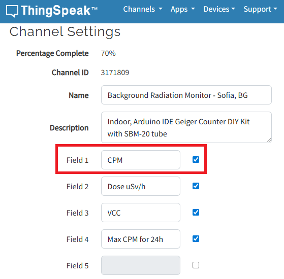
I have to say that I'm not an engineer or coder, just can simply load some Arduino sketches and few more things, so I'll be very thankfull if someone could explain like for non-IT users.
Regards,
Emo
Developing an application in MATLAB often feels like a natural choice: it offers a unified environment, powerful visualization tools, accessible syntax, and a robust technical ecosystem. But when the goal is to build a compilable, distributable app, the path becomes unexpectedly difficult if your workflow depends on symbolic functions like sym, zeta, or lambertw.
This isn’t a minor technical inconvenience—it’s a structural contradiction. MATLAB encourages the creation of graphical interfaces, input validation, and dynamic visualization. It even provides an Application Compiler to package your code. But the moment you invoke sym, the compiler fails. No clear warning. No workaround. Just: you cannot compile. The same applies to zeta and lambertw, which rely on the symbolic toolbox.
So we’re left asking: how can a platform designed for scientific and technical applications block compilation of functions that are central to those very disciplines?
What Are the Alternatives?
- Rewrite everything numerically, avoiding symbolic logic—often impractical for advanced mathematical workflows.
- Use partial workarounds like matlabFunction, which may work but rarely preserve the original logic or flexibility.
- Switch platforms (e.g., Python with SymPy, Julia), which means rebuilding the architecture and leaving behind MATLAB’s ecosystem.
So, Is MATLAB Still Worth It?
That’s the real question. MATLAB remains a powerful tool for prototyping, teaching, analysis, and visualization. But when it comes to building compilable apps that rely on symbolic computation, the platform imposes limits that contradict its promise.
Is it worth investing time in a MATLAB app if you can’t compile it due to essential mathematical functions? Should MathWorks address this contradiction? Or is it time to rethink our tools?
I’d love to hear your thoughts. Is MATLAB still worth it for serious application development?

It’s exciting to dive into a new dataset full of unfamiliar variables but it can also be overwhelming if you’re not sure where to start. Recently, I discovered some new interactive features in MATLAB live scripts that make it much easier to get an overview of your data. With just a few clicks, you can display sparklines and summary statistics using table variables, sort and filter variables, and even have MATLAB generate the corresponding code for reproducibility.
The Graphics and App Building blog published an article that walks through these features showing how to explore, clean, and analyze data—all without writing any code.
If you’re interested in streamlining your exploratory data analysis or want to see what’s new in live scripts, you might find it helpful:
If you’ve tried these features or have your own tips for quick data exploration in MATLAB, I’d love to hear your thoughts!
Pure Matlab
82%
Simulink
18%
11 voti
Title: Looking for Internship Guidance as a Beginner MATLAB/Simulink Learner
Hello everyone,
I’m a Computer Science undergraduate currently building a strong foundation in MATLAB and Simulink. I’m still at a beginner level, but I’m actively learning every day and can work confidently once I understand the concepts. Right now I’m focusing on MATLAB modeling, physics simulation, and basic control systems so that I can contribute effectively to my current project.
I’m part of an Autonomous Underwater Vehicle (AUV) team preparing for the Singapore AUV Challenge (SAUVC). My role is in physics simulation, controls, and navigation, and MATLAB/Simulink plays a major role in that pipeline. I enjoy physics and mathematics deeply, which makes learning modeling and simulation very exciting for me.
On the coding side, I practice competitive programming regularly—
• Codeforces rating: ~1200
• LeetCode rating: ~1500
So I'm comfortable with logic-building and problem solving. What I’m looking for:
I want to know how a beginner like me can start applying for internships related to MATLAB, Simulink, modeling, simulation, or any engineering team where MATLAB is widely used (including companies outside MathWorks).
I would really appreciate advice from the community on:
- What skills should I strengthen first?
- Which MATLAB/Simulink toolboxes are most important for beginners aiming toward simulation/control roles?
- What small projects or portfolio examples should I build to improve my profile?
- What is the best roadmap to eventually become a good candidate for internships in this area?
Any guidance, resources, or suggestions would be extremely helpful for me.
Thank you in advance to everyone who shares their experience!
Jorge Bernal-AlvizJorge Bernal-Alviz shared the following code that requires R2025a or later:
Test()

function Test()
duration = 10;
numFrames = 800;
frameInterval = duration / numFrames;
w = 400;
t = 0;
i_vals = 1:10000;
x_vals = i_vals;
y_vals = i_vals / 235;
r = linspace(0, 1, 300)';
g = linspace(0, 0.1, 300)';
b = linspace(1, 0, 300)';
r = r * 0.8 + 0.1;
g = g * 0.6 + 0.1;
b = b * 0.9 + 0.1;
customColormap = [r, g, b];
figure('Position', [100, 100, w, w], 'Color', [0, 0, 0]);
axis equal;
axis off;
xlim([0, w]);
ylim([0, w]);
hold on;
colormap default;
colormap(customColormap);
plothandle = scatter([], [], 1, 'filled', 'MarkerFaceAlpha', 0.12);
for i = 1:numFrames
t = t + pi/240;
k = (4 + 3 * sin(y_vals * 2 - t)) .* cos(x_vals / 29);
e = y_vals / 8 - 13;
d = sqrt(k.^2 + e.^2);
c = d - t;
q = 3 * sin(2 * k) + 0.3 ./ (k + 1e-10) + ...
sin(y_vals / 25) .* k .* (9 + 4 * sin(9 * e - 3 * d + 2 * t));
points_x = q + 30 * cos(c) + 200;
points_y = q .* sin(c) + 39 * d - 220;
points_y = w - points_y;
CData = (1 + sin(0.1 * (d - t))) / 3;
CData = max(0, min(1, CData));
set(plothandle, 'XData', points_x, 'YData', points_y, 'CData', CData);
brightness = 0.5 + 0.3 * sin(t * 0.2);
set(plothandle, 'MarkerFaceAlpha', brightness);
drawnow;
pause(frameInterval);
end
end
Parallel Computing Onramp is here! This free, one-hour self-paced course teaches the basics of running MATLAB code in parallel using multiple CPU cores, helping users speed up their code and write code that handles information efficiently.
Remember, Onramps are free for everyone - give the new course a try if you're curious. Let us know what you think of it by replying below.
Pick a team, solve Cody problems, and share your best tips and tricks. Whether you’re a beginner or a seasoned MATLAB user, you’ll have fun learning, connecting with others, and competing for amazing prizes, including MathWorks swags, Amazon gift cards, and virtual badges.
How to Participate
- Join a team that matches your coding personality
- Solve Cody problems, complete the contest problem group, or share Tips & Tricks articles
- Bonus Round: Two top players from each team will be invited to a fun code-along event
Contest Timeline
- Main Round: Nov 10 – Dec 7, 2025
- Bonus Round: Dec 8 – Dec 19, 2025
Prizes (updated 11/19)
- (New prize) Solving just one problem in the contest problem group gives you a chance to win MathWorks T-shirts or socks each week.
- Finishing the entire problem group will greatly increase your chances—while helping your team win.
- Share high-quality Tips & Tricks articles to earn you a coveted MathWorks Yeti Bottle.
- Become a top finisher in your team to win Amazon gift cards and an invitation to the bonus round.
как я получил api Token
I am excited to join this community to learn the more particularly the Matlab/Simulink
I just learned you can access MATLAB Online from the following shortcut in your web browser: https://matlab.new
Thanks @Yann Debray
From his recent blog post: pip & uv in MATLAB Online » Artificial Intelligence - MATLAB & Simulink