OptimizerSADEA

Access SADEA optimizer and its properties

Since R2025a

Description

Use the OptimizerSADEA object to create a SADEA optimizer. Use the object properties and functions set up and tune the optimizer parameters, and integrate the SADEA optimizer as a black box into your workflow using a function handle.

You can use the SADEA optimizer for moderate-dimensional global optimization problems (with 30 or fewer design variables) where function evaluations are costly. It is particularly effective for applications such as optimizing antenna designs with limited tunable parameters, wideband or multi-band antenna optimization, and multi-objective optimization.

The SADEA optimizer aims to find a local minimum of the objective function across several design variables within a bounded domain. For more information, see optimization algorithms.

Creation

Syntax

s = OptimizerSADEA(bounds)

s = OptimizerSADEA(bounds,PropertyName=Value)

Description

s = OptimizerSADEA(bounds) creates a SADEA optimizer object using default property values and the bounds specified in bounds.

s = OptimizerSADEA(bounds,PropertyName=Value) sets properties using one or more name-value arguments. PropertyName is the property name and Value is the corresponding value. You can specify the name-value arguments in any order as PropertyName1=Value1,...,PropertyNameN=ValueN. Properties that you do not specify retain their default values.

For example, s = OptimizerSADEA([1;3],UseParallel=1) creates a SADEA optimizer object with a single design variable with a lower bound of 1 and upper bound of 3 and uses a parallel pool for optimization.

Input Arguments

bounds — Lower and upper bounds of design variables

2-by-N matrix

Lower and upper bounds of the design variables, specified as a 2-by-N matrix, where N is the number of design variables for optimization. Each column represents one design variable, with the first row representing the lower bound and the second row the upper bound.

This argument sets the Bounds property.

Example: [3 0.11; 7 0.13]

Data Types: double

Properties

Bounds — Lower and upper bounds of design variables

2-by-N matrix

Lower and upper bounds of design variables, specified as a 2-by-N matrix. N is the number of design variables for optimization. Each column represents one design variable, with first row as lower bound and second row as upper bound.

Example: [3 0.11; 7 0.13]

Data Types: double

CustomEvaluationFunction — Objective of antenna or array optimization

[] (default) | custom objective function | anonymous function handle

Objective of antenna or array optimization, specified as one of these options:

• Custom objective function — Optimizes the antenna or array as per the user-defined objective function.

• Anonymous function handle — Optimizes the antenna or array for the objectives defined using the anonymous function handle.

Example: @MinimizeArraySpacing

Data Types: function_handle

Weights — Weight or penalty of each constraint function

[] (default) | vector of positive integers in the range (0,100]

Weight or penalty of each constraint function, specified as a vector of positive integers in the range (0,100]. The summation of all the weights must be 100. If you specify a high value, the function gives a higher priority to the constraint when optimizing multiple constraints.

When optimizing multiple constraints, the function prioritizes constraint functions based on the weights.

Example: [20 50 30]

Data Types: double

UseParallel — Option to enable parallel pool

0 (default) | 1

Option to enable parallel pool, specified as a logical value. The default value is 0. Set this option to 1 to enable the parallel pool. Use parallel pool to speed up the optimization for computationally large antennas and arrays, or in case of high number of design variables. To use this feature, you need a license for Parallel Computing Toolbox™.

Use the canUseParallelPool function to check if Parallel Computing Toolbox is installed and licensed for use, a default parallel pool is configured and supported, and automatic creation of parallel pools is enabled.

Example: 1

Data Types: logical

GeometricConstraints — Geometric constraints

1-by-1 structure (default) | structure

Geometric constraints for optimization, specified as a structure of coefficient matrix and constant vector.

Specify linear inequality constraints in the A matrix and b vector.

• A is a real M-by-N matrix, where M is the number of inequalities, and N is the number of design variables. A holds the design variable coefficients of the inequalities.

• b is a real M-element column vector and holds the constants of inequalities corresponding to the coefficients in A.

For example, consider an optimization problem consisting of five design variables as follows:

designVariables = {'CenterArmNotchLength','NotchLength','Width',...
            'CenterArmNotchWidth','NotchWidth'};

The geometric constraints for optimization are:

• 5*CenterArmNotchLength - NotchLength < 0

• CenterArmNotchWidth + 2*Notchwidth - Width < 0

Define the A and b as follows:

A = [5,-1,0,0,0;...
     0,0,-1,1,2];
b = [0;0];

Specify linear equality constraints in the Aeq matrix and beq vector.

• Aeq is an Me-by-N matrix, where Me is the number of equalities, and N is the number of design variables. Aeq holds the design variable coefficients of the equalities.

• beq is a real Me-element column vector and holds the constants of equalities corresponding to the coefficients in Aeq.

Specify nonlinear inequality constraints in the nlcon matrix and nrlv vector.

• nlcon is a function handle that defines nonlinear constraints. It stores the design variables.

• nrlv is a 1-by-N vector of 0 and 1. N is the number of design variables in nlcon. Each element in nrlv represents an index and corresponds to a design variable in nlcon in the same sequence as nlcon. Specify 1 to convey to the optimize function that the corresponding design variable is relevant for optimization. Specify 0 to convey to the optimize function that the corresponding design variable is not relevant for optimization.

For example, to maximize the gain of a dipole antenna operating at 75 MHz with constraints on its length and width, use this code:

optAnt = OptimizerSADEA([1 4; 3 7]);
optAnt = OptimizerSADEA(GeometricConstraints=opt);
opt = 

  struct with fields:

        A: [100×2 double]
        b: [100×1 double]
      Aeq: [-1 5]
      beq: 0
    nlcon: @btw
     nrlv: [1 1]

For additional information on linear and nonlinear equalities and nonlinear inequalities, see the fmincon (Optimization Toolbox) function documentation.

Example: A=[5,-1,0,0,0; 0,0,-1,1,2]; b=[0;0]; structure.A=A; structure.b=b;

Example: Aeq=[-1 5]; beq=0; structure.Aeq=Aeq; structure.beq=beq;

Example: nlcon=@btw; nrlv=[1 1]; structure.nlcon=nlcon; structure.nrlv=nrlv;

Data Types: struct

EnableLog — Option to print iteration number and value of convergence at command line

0 (default) | 1

Option to print iteration number and value of convergence at the command line, specified as a logical 1 to enable or 0 to disable. By default, this option is disabled.

Example: 1

Data Types: logical

Object Functions

checkExitCondition	Check exit status of optimizer
defineInitialPopulation	Set initial population size
getBestMemberData	View best member data after optimization
getInitializationData	View optimizer member data at initialization
getIterationData	View optimization data for completed iterations
getNumberOfEvaluations	Get number of function evaluations performed
isConverged	Check convergence status of optimizer
isFunctionEvaluationsExhausted	Check function evaluations completion status
optimize	Optimize custom evaluation function using specified parameters
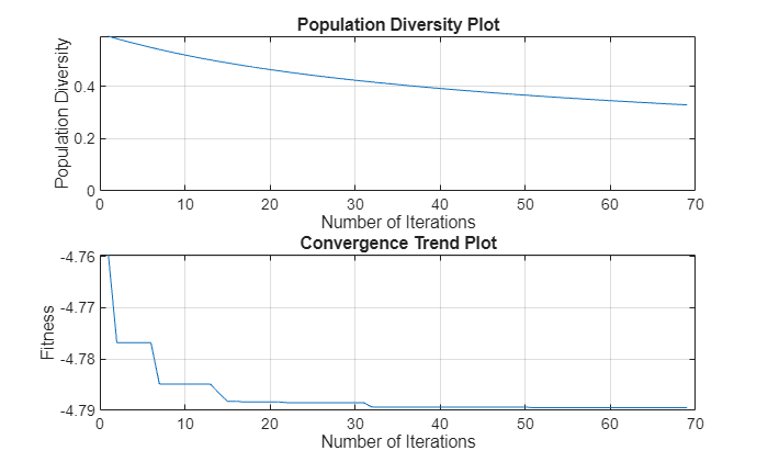
optimizeWithPlots	Optimize custom evaluation function and plot population density and convergence
performRestore	Restore optimizer parameters to values from the previous successful iteration
setMaxFunctionEvaluations	Set upper limit for number of function evaluations
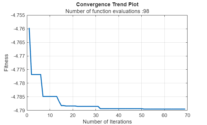
showConvergenceTrend	Plot optimization convergence trend

Examples

Optimize Dipole Antenna for Directivity

Create a dipole antenna resonating at 75 MHz and calculate its maximum directivity.

Choose its length and width as design variables. Provide lower and upper bounds of length and width.

referenceAnt = design(dipole,75e6);
InitialDirectivity = max(max(pattern(referenceAnt,75e6)))

InitialDirectivity = 
2.1002

Bounds = [3 0.11; 7 0.13];

Use the SADEA optimizer to optimize this dipole antenna for its directivity. Specify an evaluation function for optimization using the CustomEvaluationFunction property of the OptimizerSADEA object. The evaluation function used in this example is defined at the end of this example.

s = OptimizerSADEA(Bounds);
s.CustomEvaluationFunction = @customEvaluationOnlyObjective;

Run the optimization for 100 iterations.

figure
s.optimizeWithPlots(100);

View the best member data.

bestDesign = s.getBestMemberData

bestDesign = 
  bestMemberData with properties:

             member: [4.7998 0.1101]
       performances: -4.7895
            fitness: -4.7895
    bestIterationId: 50

bestdesignValues = bestDesign.member

bestdesignValues = 1×2

    4.7998    0.1101

Update the reference antenna with best design values from the optimizer. Calculate directivity of the optimized design.

Observe an increase in directivity value after optimization.

referenceAnt.Length = bestdesignValues(1);
referenceAnt.Width = bestdesignValues(2);
postOptimizationDirectivity = max(max(pattern(referenceAnt,75e6)))

postOptimizationDirectivity = 
4.7895

View the surrogate model data used for prediction.

InitialData = s.getInitializationData

InitialData = 
  initializationData with properties:

         members: [30×2 double]
    performances: [30×1 double]
         fitness: [30×1 double]

View the data for all iterations.

iterData = s.getIterationData

iterData = 
  iterationData with properties:

         members: [68×2 double]
    performances: [68×1 double]
         fitness: [68×1 double]

Check if the algorithm has converged.

ConvergenceFlag = s.isConverged

ConvergenceFlag = logical
   1

Check how many times the evaluation function is computed.

NumEvaluations = s.getNumberOfEvaluations

NumEvaluations = 
98

Plot the convergence trend.

s.showConvergenceTrend

Following code defines the evaluation function used in this example.

function fitness = customEvaluationOnlyObjective(designVariables)
    fitness = [];
    try
        % Create geometry
        ant = design(dipole,75e6);
        ant.Length = designVariables(1);
        ant.Width = designVariables(2);
    catch
        % Handle errors during geometry creation.
        % High penalty value is used to handle errors.
        fitness = 1e6;
    end
    
    if isempty(fitness)
        try
            % Calculate directivity
            % Optimizer always minimizes the objective hence reverse the sign to maximize gain.
            objective = max(max(pattern(ant,75e6)));
            objective = -objective; 
        catch
            % Handle errors during gain computation.
            % High penalty value is used to handle errors.
            objective = 1e6;
        end
        % As there are no constraints, fitness equals objective.
        fitness = objective;
    end
end

Version History

Introduced in R2025a