optimize

Optimize custom evaluation function using specified parameters

Since R2025a

Syntax

opt = optimize(obj,iterations)

Description

opt = optimize(obj,iterations) optimizes the custom evaluation function specified in the optimizer obj using the number of iterations in iterations.

Examples

Optimize Reflector Antenna for Directivity

Create a four-element linear array of dipole antennas. Use it as an exciter for a reflector antenna.

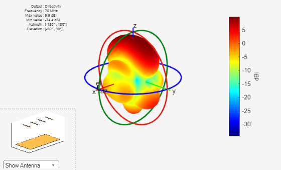
Calculate maximum directivity of this reflector antenna.

la = linearArray(NumElements=4);
la.Tilt = 90;
referenceAnt = reflector;
referenceAnt.Exciter = la;
referenceAnt.GroundPlaneLength = 8;
referenceAnt.GroundPlaneWidth = 4;
referenceAnt.Spacing = 4;
InitialDirectivity = max(max(pattern(referenceAnt,70e6)))

InitialDirectivity = 
9.9028

figure
pattern(referenceAnt,70e6)

Find the lowest return loss among all ports of this antenna at 70 MHz.

freq = 70e6;
sp = sparameters(referenceAnt,freq);
RetLossPort1 = 20*log10(max(abs(rfparam(sp,1,1))));
RetLossPort2 = 20*log10(max(abs(rfparam(sp,2,2))));
RetLossPort3 = 20*log10(max(abs(rfparam(sp,3,3))));
RetLossPort4 = 20*log10(max(abs(rfparam(sp,4,4))));
InitialLowestRetLossVal = max([RetLossPort1,RetLossPort2,RetLossPort3,RetLossPort4]);

Choose spacing between the dipoles of the exciter and exciter to reflector spacing as design variables. Specify the lower and upper bounds of these design variables.

Use the TR-SADEA optimizer to optimize this reflector antenna for its directivity and return loss. Specify an evaluation function for optimization using the CustomEvaluationFunction property of the OptimizerTRSADEA object. The evaluation function used in this example is defined at the end of this example.

Set the maximum number of function evaluations to 90 and initial population sample size to 10. Setting these parameters is optional. The TR-SADEA optimizer calculates best sample size automatically if you do not specify it.

Bounds = [0.1 0.1; 10 10];
s = OptimizerTRSADEA(Bounds);
s.CustomEvaluationFunction = @customEvaluationWithConstraint2;
setMaxFunctionEvaluations(s,90);
defineInitialPopulation(s,10);

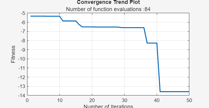
Run optimization for 50 iterations and check if maximum function evaluations have been reached. Observe the convergence trends plot.

optimize(s,50);
flag0 = isFunctionEvaluationsExhausted(s)

flag0 = logical
   0

showConvergenceTrend(s) 

View the best member data.

bestDesign = s.getBestMemberData

bestDesign = 
  bestMemberData with properties:

             member: [2.2926 2.8495]
       performances: -13.5865
            fitness: -13.5865
    bestIterationId: 41

bestdesignValues = bestDesign.member

bestdesignValues = 1×2

    2.2926    2.8495

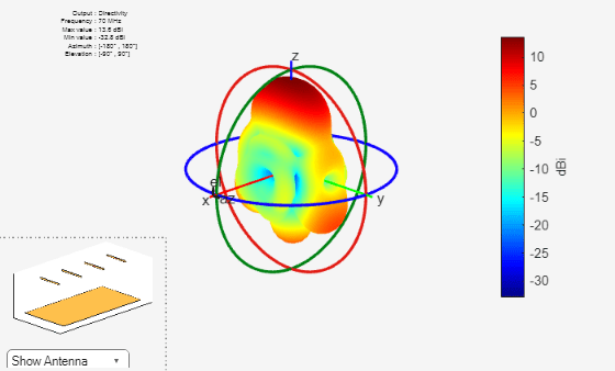
Update reference antenna with the design values obtained from the optimization and calculate the directivity.

Observe the increase in directivity post optimization.

referenceAnt.Exciter.ElementSpacing = bestdesignValues(1);
referenceAnt.Spacing = bestdesignValues(2);
postOptimizationDirectivity = max(max(pattern(referenceAnt,70e6)))

postOptimizationDirectivity = 
13.5865

figure
pattern(referenceAnt,70e6)

Calculate the post optimization return loss. Use the lowest return loss value among all ports.

Observe that the value of return loss after optimization is better than its previous value.

sp = sparameters(referenceAnt,freq);
RetLossPort1 = 20*log10(max(abs(rfparam(sp,1,1))));
RetLossPort2 = 20*log10(max(abs(rfparam(sp,2,2))));
RetLossPort3 = 20*log10(max(abs(rfparam(sp,3,3))));
RetLossPort4 = 20*log10(max(abs(rfparam(sp,4,4))));
NewLowestRetLossVal = max([RetLossPort1,RetLossPort2,RetLossPort3,RetLossPort4]);

Check the exit status of the optimizer.

flag1 = isFunctionEvaluationsExhausted(s)

flag1 = logical
   0

flag2 = checkExitCondition(s)

flag2 = logical
   0

Restore the optimizer parameters to their previous successful iteration values. Use this step if the current iteration is interrupted and the iteration data is incomplete.

res = performRestore(s)

res = 
  OptimizerTRSADEA with properties:

                      Bounds: [2×2 double]
    CustomEvaluationFunction: @customEvaluationWithConstraint2
                     Weights: []
                 UseParallel: 0
        GeometricConstraints: [1×1 struct]
                   EnableLog: 0

Following code defines the evaluation function used in this example.

function fitness = customEvaluationWithConstraint2(designVariables)
    fitness = [];
    try
        % Create geometry
        la = linearArray(NumElements=4);
        la.Tilt = 90;
        la.ElementSpacing = designVariables(1);
        r = reflector;
        r.Exciter = la;
        r.GroundPlaneLength = 8;
        r.GroundPlaneWidth = 4;
        r.Spacing = designVariables(2);
    catch
        % Handle errors during geometry creation
        % High penalty value is used to handle errors
        fitness = 1e6;
    end
    
    if isempty(fitness)
        try
            % Calculate realized gain 
            objective = max(max(pattern(r, 70e6)));
            objective = -objective; % As optimizer always minimizes objective, 
            % sign is reversed to maximize gain.
        catch
            % Handle errors during gain computation
            % High penalty value is used to handle errors
            objective = 1e6;
        end
    
        try
            % Constraints s11 < -10
            % Calculate S-parameters
            freq = 70e6;
            s = sparameters(r,freq);
            RetLossPort1 = 20*log10(max(abs(rfparam(s,1,1))));
            RetLossPort2 = 20*log10(max(abs(rfparam(s,2,2))));
            RetLossPort3 = 20*log10(max(abs(rfparam(s,3,3))));
            RetLossPort4 = 20*log10(max(abs(rfparam(s,4,4))));
            lowestRetLossVal = max([RetLossPort1,RetLossPort2,RetLossPort3,RetLossPort4]);
            expVal = -20;
            % As constraint is satisfied when it is less than -20 dB, better
            % values are made to be equal to -20 dB to not affect optimizer
            % direction.
            constraint = (lowestRetLossVal-expVal);
            constraint = max(constraint,0);
        catch
            % Handle errors during S-parameters computation.
            % High penalty value is used to handle errors.
            constraint = 1e6;
        end
        fitness = objective + constraint;
    end
end

Input Arguments

obj — Optimizer

OptimizerSADEA object | OptimizerTRSADEA object

Optimizer, specified as an OptimizerSADEA or OptimizerTRSADEA object. The function optimizes the custom evaluation function associated with the optimizer object specified in obj.

Example: OptimizerSADEA

iterations — Number of iterations for optimization

positive integer

Number of iterations for optimization, specified as a positive integer.

Example: 100

Data Types: double

Output Arguments

opt — Optimized custom evaluation function parameters

OptimizerSADEA object | OptimizerTRSADEA object

Optimized custom evaluation function parameters, returned as an OptimizerSADEA or OptimizerTRSADEA object. Use the getBestMemberData function to access the optimization results.

Version History

Introduced in R2025a