Design Hard-Disk Read/Write Head Controller
This example shows how to design a computer hard-disk read/write head position controller using classical control design methods.
Create Read/Write Head Model
Using Newton's laws, model the read/write head using the following differential equation:
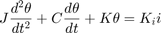
Here,
 is the inertia of the head assembly.
 is the viscous damping coefficient of the bearings.
 is the return spring constant.
 is the motor torque constant.
 is the angular position of the head.
 is the input current.
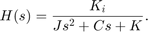
Taking the Laplace transform, the transfer function from to is
Specify the physical constants of the model, such that:


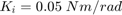
J = 0.01;
C = 0.004;
K = 10;
Ki = 0.05;
Define the transfer function using these constants.
num = Ki;
den = [J C K];
H = tf(num,den)
H =

           0.05
  -----------------------
  0.01 s^2 + 0.004 s + 10

Continuous-time transfer function.
Discretize the Model
To design a digital controller that provides accurate positioning of the read/write head, first discretize the continuous-time plant.
Specify the sample time.
Ts = 0.005;
Discretize the model. Since the controller will have a digital-to-analog converter (with a zero-order hold) connected to its input, use the c2d command with the 'zoh' discretization method.
Hd = c2d(H,Ts,'zoh')
Hd =

  6.233e-05 z + 6.229e-05
  -----------------------
   z^2 - 1.973 z + 0.998

Sample time: 0.005 seconds
Discrete-time transfer function.
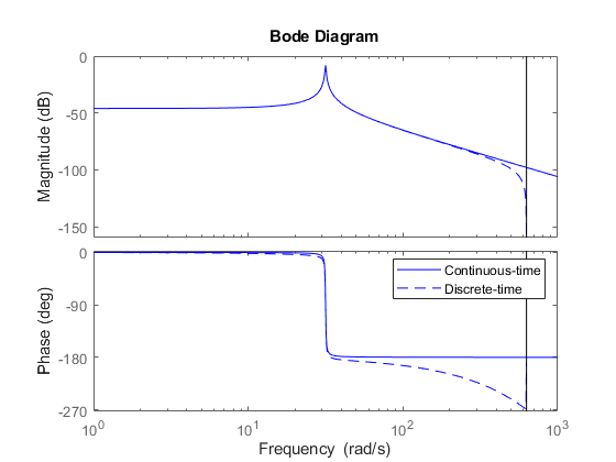
Compare the Bode plots of the continuous-time and discrete-time models.
bodeplot(H,'-',Hd,'--')
legend('Continuous-time','Discrete-time')
To analyze the discretized system, plot its step response.
stepplot(Hd)
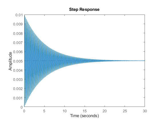
The step response has significant oscillation, which is most likely due to light damping. Check the damping for the open-loop poles of the system.
damp(Hd)
         Pole             Magnitude     Damping       Frequency      Time Constant
                                                    (rad/seconds)      (seconds)

  9.87e-01 + 1.57e-01i     9.99e-01     6.32e-03       3.16e+01         5.00e+00
  9.87e-01 - 1.57e-01i     9.99e-01     6.32e-03       3.16e+01         5.00e+00
As expected, the poles have light equivalent damping and are near the unit circle. Therefore, you must design a compensator that increases the damping in the system.
Add a Compensator Gain
The simplest compensator is a gain factor with no poles or zeros. Try to select an appropriate feedback gain using the root locus technique. The root locus plots the closed-loop pole trajectories as a function of the feedback gain.
rlocus(Hd)
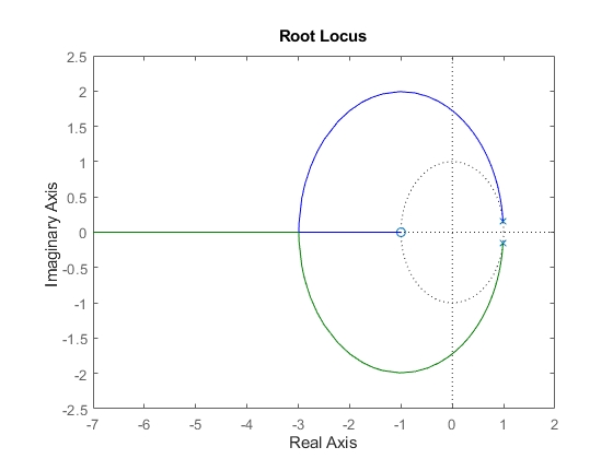
The poles quickly leave the unit circle and go unstable. Therefore, you must introduce some lead to the system.
Add a Lead Network
Define a lead compensator with a zero at  and a pole at
  .
.

D = zpk(0.85,0,1,Ts);
The corresponding open-loop model is the series connection of the compensator and plant.
oloop = Hd*D
oloop =

  6.2328e-05 (z+0.9993) (z-0.85)
  ------------------------------
     z (z^2 - 1.973z + 0.998)

Sample time: 0.005 seconds
Discrete-time zero/pole/gain model.
To see how the lead compensator affects the open-loop frequency response, compare the Bode plots of Hd and oloop.
bodeplot(Hd,'--',oloop,'-')
legend('Plant','Plant plus lead compensator')
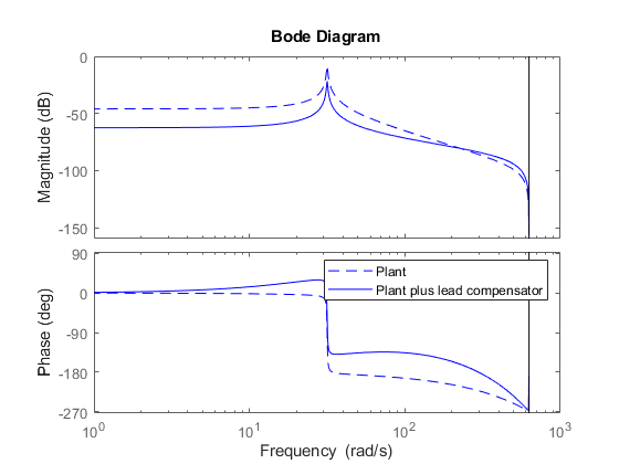
The compensator adds lead to the system, which shifts the phase response upward in the frequency range  .
.
Examine the behavior of the closed-loop system poles using a root locus plot. Set the limits of both the x-axis and y-axis from -1 to 1.
rlocus(oloop)
grid
xlim([-1 1])
ylim([-1 1])
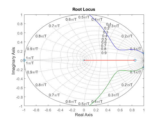
The closed-loop poles now remain within the unit circle for some time.
To create a data marker for the plot, click the root locus curve. Find the point on the curve where the damping is greatest by dragging the marker. The maximum damping of 0.782 corresponds to a feedback gain of 4.07e+03.
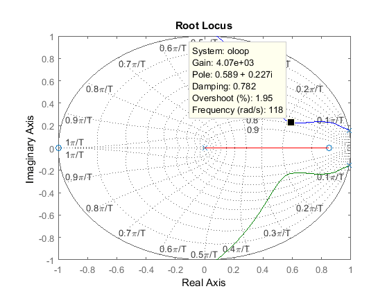
Analyze Design
To analyze this design, first define the closed-loop system, which consists of the open-loop system with a feedback gain of 4.07e+03.
k = 4.07e+03;
cloop = feedback(oloop,k);
Plot the closed-loop step response.
stepplot(cloop)
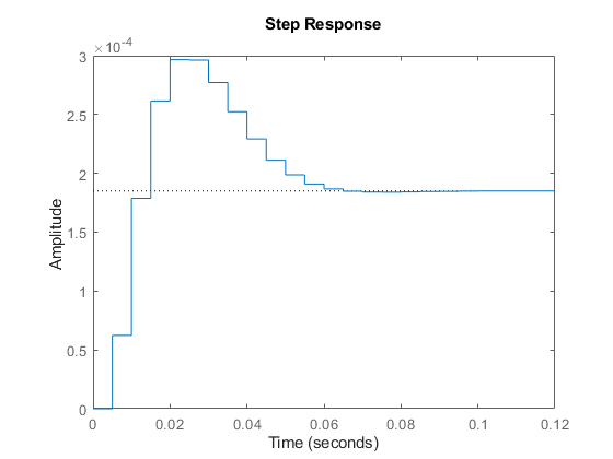
This response depends on your closed-loop setpoint. The one shown here is relatively fast and settles in about 0.06 seconds. Therefore, the closed-loop disk drive system has a seek time of 0.06 seconds. While this seek time is relatively slow by modern standards, you also started with a lightly-damped system.
It is good practice to examine the robustness of your design. To do so, compute the gain and phase margins for your system. First, form the unity feedback open-loop system by connecting the compensator, plant, and feedback gain in series.
olk = k*oloop;
Next, compute the margins for this open-loop model.
[Gm,Pm,Wcg,Wcp] = margin(olk)
Gm =

    3.8360


Pm =

   43.3061


Wcg =

  296.7988


Wcp =

  105.4736
This command returns the gain margin, Gm, the phase margin Pm, and their respective cross-over frequencies, Wcg and Wcp.
Convert the gain margin to dB.
20*log10(Gm)
ans =

   11.6776
You can also display the margins graphically.
margin(olk)
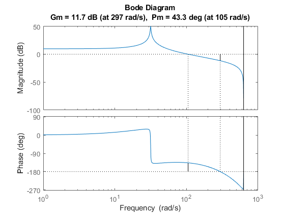
This design is robust and can tolerate an 11-dB gain increase or a 40-degree phase lag in the open-loop system without going unstable. By continuing this design process, you may be able to find a compensator that stabilizes the open-loop system and reduces the seek time further.