CBRS Band Radar Parameter Estimation Using YOLOX

This example shows how to detect rectangular-pulse and linear-FM radar waveforms in noise and estimate their time and frequency characteristics using a combination of time-frequency maps and a deep learning object detector. Specifically, the example uses a pooled version of the spectrogram and a You Only Look Once X (YOLOX) object detector. For an introduction to the YOLOX object detector, see Getting Started with YOLOX for Object Detection (Computer Vision Toolbox). YOLOX requires the Automated Visual Inspection Library for Computer Vision Toolbox.

Spectrum Sensing for Radar Data

Radar data is increasingly required to share bandwidth with mobile broadband signals. One example of this in the United States is the Citizens Broadband Radio Service (CBRS). CBRS is a 150 MHz-wide portion of the 3.5 GHz band that the US Federal Communications Commission opened up to commercial use in 2017. The band had been previously reserved for government radar and some satellite communications. Increasingly, it is not feasible to reserve portions of the spectrum solely for radar use. As a result, radar transmissions cannot be expected to remain free from interfering signals. This requires us to develop effective spectrum sensing techniques, which can detect and classify radar signals as well as estimate their time-bandwidth parameters without the benefit of any knowledge of the transmitter's characteristics. In the modern radio-frequency environment, a sensor can be expected to be impinged on by a wide variety of radar and cellular signals with different spectral characteristics. Because the sensor has no knowledge of the transmitter's characteristics, the use of a matched filter to enhance the radar signal's SNR is not feasible. This makes accurate detection of radar signals in unfavorable SNR conditions extremely challenging. Modern deep-learning object detectors trained on real-world images offer the potential to help in this task by training the object detectors on images obtained from time-frequency representations of radar signals.

Data

The data in this example are simulations of both rectangular-pulsed and linear-FM radar signals in noise generated using Simulated Radar Waveform and RF Dataset Generator for Incumbent Signals in the 3.5 GHz CBRS Band. This MATLAB® software was also used to create the freely available RF Dataset of Incumbent Radar Systems in the 3.5 GHz CBRS Band [1]. The data set used in this example for training and validation consists of 800 simulated radar waveforms in additive complex-valued white Gaussian noise. The data are sampled at 10 MHz. Each waveform is 160,000 samples long and represents 0.016 seconds of data. There are 400 rectangular-pulse radar waveforms labeled P0N#1 and 400 linear-FM pulse waveforms labeled Q3N#3. The labels P0N#1 and Q3N#3 are used for consistency with the 3.5 GHz CBRS Band data set previously referenced. These are also the labels used by the software that generated the data for this example. For both pulse types, the radar signals always start at 0.002 seconds (20,000 samples). To generate the rectangular-pulse waveforms, the software uses phased.RectangularWaveform with parameterizations chosen randomly from the following:

• Pulse width: 0.5 to 2.5 microseconds

• Pulse repetition frequency: 900 to 1100 Hz

• Number of Pulses: 15 to 40

To generate the linear-FM pulse waveforms, the software uses phased.LinearFMWaveform with random parameterizations from these ranges:

• Pulse width: 50 to 100 microseconds

• Pulse repetition frequency: 300 to 3000 Hz

• Chirp width: 50 to 100 MHz

• Chirp direction: up and down

• Envelop: rectangular

Fix the sweep interval to "Symmetric". Complex-valued white Gaussian noise is added to create waveforms with randomly chosen SNRs between 17 and 20 dB. Resample all waveforms to have a total bandwidth of 10 MHz using a Kaiser window lowpass filter with a shape parameter value of 10.

Download the data set. The unzipped data requires about 2.1 GB of disk space. When unzipped, there is a license.txt file containing information about licensing and two folders traindata and testdata, containing the training data and testing data with a pre-trained model.

datasetZipFile = matlab.internal.examples.downloadSupportFile("SPT","data/RPLFMSimulatedRadarDataset.zip");
datasetFolder = fullfile(fileparts(datasetZipFile),"RPLFMSimulatedRadarDataset"); 
if ~exist(datasetFolder,"dir") 
    unzip(datasetZipFile,datasetFolder); 
end

Load the training data.

load(fullfile(datasetFolder,"traindata","RPFMradardataTrain.mat"));
load(fullfile(datasetFolder,"traindata","RPFMradardataTrainLabels.mat"));
load(fullfile(datasetFolder,"traindata","RPFMradardataTrainmetaData.mat"));

First show that there are an equal number of waveforms in the two categories.

summary(RPFMradardataTrainLabels)

RPFMradardataTrainLabels: 800×1 categorical

     P0N#1            400 
     Q3N#3            400 
     <undefined>        0 

Next, select one rectangular-pulse and one linear-FM radar waveform at random from the data. Plot the real- and imaginary parts along with magnitudes. Designate the rectangular-pulse waveform as "RP" and the linear-FM waveform as "FM".

rng("default")
idxPW = find(RPFMradardataTrainLabels == categorical("P0N#1"));
idxFM = find(RPFMradardataTrainLabels==categorical("Q3N#3"));
selectidx = randi([1 400]);
RPWave = RPFMradardataTrain(:,idxPW(selectidx));
RPSNR = RPFMradardataTrainmetaData{idxPW(selectidx),"SNR"};
FMSNR = RPFMradardataTrainmetaData{idxFM(selectidx),"SNR"};
FMWave = RPFMradardataTrain(:,idxFM(selectidx));
fs = 1e7;
t = 0:1/fs:(160000*1/fs)-1/fs;
tiledlayout(3,2)
ax1 = nexttile;
plot(t,real(RPWave))
title(["RP Waveform (Real Part)" ; "SNR = " + num2str(RPSNR)]);
ax1(1).XTickLabel = [];
ylabel("Amplitude")
ax2 = nexttile;
plot(t,real(FMWave))
title(["FM Waveform (Real Part)" ; "SNR = " + num2str(FMSNR)]);
ax2.XTickLabel = [];
nexttile
plot(t,imag(RPWave))
title("RP Waveform (Imaginary Part)");
ylabel("Amplitude")
ax3 = nexttile;
plot(t,imag(FMWave))
title("FM Waveform (Imaginary Part)");
ax3.XTickLabel = [];
nexttile
plot(t,abs(RPWave))
title("RP Waveform (Magnitude)");
ylabel("Magnitude")
xlabel("Seconds")
nexttile
plot(t,abs(FMWave))
title("FM Waveform (Magnitude)");
xlabel("Seconds")

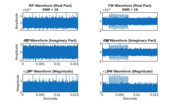
While it is possible in this example to visualize the pulses in the linear-FM waveform, it is difficult to reliably discern the rectangular pulses in the presence of noise in the time domain.

YOLO-like Object Detection in Radar

Before delving into the details of the example, it is helpful to first explain what we mean by object detection in a YOLO context as it relates specifically to radar detection and estimation. It is important to note that object detection in YOLO networks combines both detection and estimation, or to use machine-learning language, classification and regression. YOLOX, like other YOLO networks, is a single-stage detector that looks at an image once to both determine if objects are present, what type of object is present, and what are the locations of those objects. In a radar application, the image is a time-frequency representation of the radar signal. There are various ways to transform a 1-D radar signal to a 2-D image-like representation. This examples uses a modification of the short-time Fourier transform (STFT), but the regression, or parameter estimation, aspect of YOLOX only depends on being able to map image coordinates to physical characteristics of the radar signal. Accordingly, other time-frequency representations can also serve as inputs for a YOLOX network.

YOLOX does not divide the image into fixed grid sizes for identifying potential objects. Rather, YOLOX uses a multiresolution approach to generate multiscale feature maps. These features are used to produce the 3 outputs of the network:

• Classes of the detected object. In a radar context, this corresponds to the type of radar signal detected, e.g. rectangular pulse, Barker code, FM waveform. This is the classification, or detection, part of the network.

• Bounding boxes for the object. In a radar context, this can be used to determine the onset time of the pulse, the duration of the pulse, the frequency offset of the pulse, and its bandwidth. This is the regression or radar signal parameter estimation part of the network. As the user, you must know how to relate the image coordinates returned by the network to the physical characteristics of the signal.

• Objectness scores of the bounding boxes. This uses intersection over union (IoU) during training to assess how well the estimated bounding box overlaps with the ground-truth. The more the estimated bounding box overlaps with the ground-truth bounding box the higher the IoU score. Based on training, the detector develops its own sense of objectness, which is then used at inference when the ground-truth is not available and IoU cannot be computed. There may be some confusion between the class of the detected object and object confidence score. They are independent terms in the YOLOX loss function.

Finally, the class probability is multiplied by the objectness score to obtain the final confidence score for each detected object belonging to a specific class. These outputs are discussed further in Radar Parameter Estimation and Noise-Only Signals.

Max-Pooled Spectrogram

This example uses max-pooled spectrograms as images for the YOLOX object detector. Reference [2] obtains the frequency-centered power spectrogram in dB of the baseband I-Q waveforms using a rectangular window with a length corresponding to 16 samples (1.6 microseconds). An overlap of 0 samples is used between adjacent windows. The window length of 1.6 microseconds is justified based on the fact that radar pulses are typically much shorter in duration than any potentially interfering noise or mobile communications signals. This results in a spectrogram with dimensions 10000-by-16 if we have frequency along the column dimension and time segment along the row dimension. Note in image coordinates, frequency represents the x-dimension and time the y-dimension. This highly rectangular aspect ratio is suboptimal for use in YOLO networks. Further, given the computational complexity of YOLO networks, an image size of 1000 along one of the spatial dimensions significantly increases the computational burden for training and inference. Accordingly, the authors in [2] achieve a further reduction of the spectrogram by grouping the 16-sample windows in blocks of 32 and taking the maximum value over the 16 frequency bins. We use the term max-pooled spectrogram to describe the effect of this operation because it is a max-pooling operation over frequency. This results in a spectrogram image with dimensions 312-by-16. Note the final 256 samples of the waveform are discarded because 512 does not divide 10000. The rationale for grouping the spectrogram into (32)(16)(1e-7)=51.2 microsecond windows for the pooling operation is that the inter-pulse intervals in the NIST RF dataset range from 0.3 msec to 3.3 msec. The value of 51.2 microseconds ensures that two radar pulses do not fall in the same pooling operation. For more detail, see table II in [2]. The authors use the resulting images of size 312-by-16 as inputs to a custom YOLO-like network they term RadYOLO. Max pooling the spectrogram in this way not only produces image aspect ratios more amenable to analysis with YOLO-type networks, it also aids in the discriminability of the radar objects in the presence of noise. The latter advantage is illustrated in the following code, which uses the helper function, maxpooledSTFT.

[Spooled,Sunpooled,f,T] = maxpooledSTFT(RPFMradardataTrain(:,2),128,32, ...
    rectwin(16),Scaling="db");
tiledlayout(1,2)
nexttile
imagesc(f./1e6,1:size(Spooled,1),Spooled)
title("Max-Pooled Spectrogram")
ylabel("Time Slot (51.2 microsecond intervals)")
xlabel("Frequency (MHz)")
nexttile
imagesc(f./1e6,T,Sunpooled')
title("Spectrogram")
ylabel("Time (seconds)")
xlabel("Frequency (MHz)")

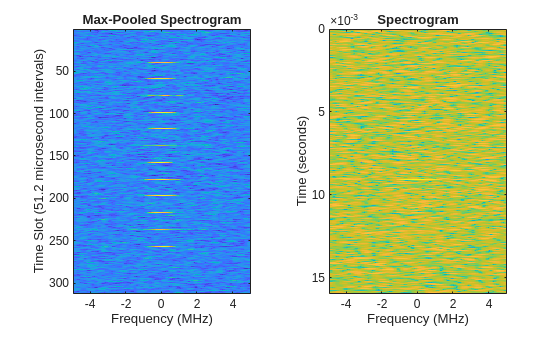
Note that in the max-pooled spectrogram, the rectangular pulses centered around zero frequency (DC) are evident, while in the spectrogram without pooling they are barely, if at all, discernable. In the code above, you can change the scaling from dB to the magnitude ("mag") or squared magnitude ("sqmag") to see the effect of this pooling with other normalizations.

While pooling the spectrogram aids in the discernability of the radar pulses in the presence of noise, it does cause two complications in the time localization of the radar pulses. The first one is simply due to the reduction in time resolution from the pooling of the spectrogram. In this case, each successive time slot in the pooled spectrogram has a duration of 51.2 microseconds. This loss of precise time localization is no different than what one encounters in the normal use of the STFT in most applications and is not a major concern. The second challenge concerns the interaction between the loss of time resolution and the downsampling and pooling within the YOLOX network. Due to the typical short time duration of radar pulses, the pulse occupies a very small number of pixels in y-dimension of the image (recall here that time is along the image y-coordinate). Assume that there is no pooling of the spectrogram and a time window of 16 samples is used with no overlap. Those 16 samples constitute 1.6 microseconds of time and one pixel along the y-dimension of the image. Examine the distribution of pulse widths for both classes in the training data.

figure
tiledlayout(2,1)
nexttile
histogram(RPFMradardataTrainmetaData{string(RPFMradardataTrainmetaData{:,"BinNo"}) == "P0N#1",'PulseWidth'}./1e-6)
ylabel('Frequency')
title("Rectangular Pulse -- Pulse Widths")
nexttile
histogram(RPFMradardataTrainmetaData{string(RPFMradardataTrainmetaData{:,"BinNo"}) == "Q3N#3",'PulseWidth'}./1e-6)
title("Linear FM Pulse -- Pulse Widths")
xlabel('Microseconds')
ylabel('Frequency')

Without pooling, the rectangular pulses only occupy a pixel or two in the y-dimension of the image. In YOLOX, the h-coordinate corresponds to the spread along time. Even the small amount of pooling used in this example, reduces h-coordinate to less than a pixel. In terms of the YOLOX network architecture, this problem is exacerbated by downsampling and pooling in the network. In Training YOLOX on Max-pooled Spectrograms and Radar Parameter Estimation and Noise-Only Signals, we discuss some mitigation strategies, but these do not obviate the difficulty in accurately estimating the actual radar pulse duration from the h-coordinate of the bounding box estimated by YOLOX.

Data Preparation

To train a YOLOX network on the radar data, first compute the ground-truth bounding boxes on the training data. To specify a bounding box use [x,y,w,h] coordinates. For the max-pooled spectrogram images, the x-coordinate represents the starting frequency in terms of discrete Fourier transform (DFT) bins from -Fs/2 to Fs/2. In this example, we use 128 DFT bins so the spacing between DFT bins is 1e7/128. The y-coordinate represents time in terms of the time windows used in the pooled spectrogram, which has physical units of 32*16*1e-7 seconds. Accordingly, each increment in the y-coordinate represents 51.2 microseconds. The w-coordinate denotes the spectral extent of the pulse in DFT bins, and the h-coordinate represents the spread in time.

In order to manage the bounding box computation and the creation of training and validation sets, use datastores. The following code creates a CombinedDatastore object that outputs a radar waveform, its label, and its metadata for each read.

traindatacell = mat2cell(RPFMradardataTrain,160e3,ones(size(RPFMradardataTrain,2),1))';
sdsTrain = signalDatastore(traindatacell);
lbldsTrain = arrayDatastore(RPFMradardataTrainLabels);
metadataDSTrain = arrayDatastore(RPFMradardataTrainmetaData);
cds = combine(sdsTrain,lbldsTrain,metadataDSTrain);

Split the data into training and validation sets. Allocate 70% of the observations to the training set and the remaining 30% to the validation set.

rng("default")
idxsplt = splitlabels(cds,0.7,"randomized",underlyingDatastoreIndex=2);
trainDS = subset(cds,idxsplt{1});
valDS = subset(cds,idxsplt{2});

To compute the ground-truth bounding boxes, use the helper function, maxpooledSTFTwithBoundingBoxes. In training a YOLO network, the deep network must be provided with the image, the ground-truth bounding boxes, and the labels for each bounding box. This information is packaged in a 1-by-3 cell array. The helper function, maxpooledSTFTwithBoundingBoxes, computes the max-pooled short-time Fourier transform (STFT) power in dB using a rectangular window length of 16 samples and pads the Fourier transform to length 128. There is no overlap between adjacent windows. The STFT power in dB is pooled over 32 windows of length 16, for a pooling interval of 51.2 microseconds to mimic the use of the max-pooled STFT power in [2]. Because the YOLOX network used in this example requires 3-channel images, the function replicates each page of the image to form three channels.

To mitigate the effect of the small time extent of the radar pulses discussed in Max-Pooled Spectrogram, we add 3 pixels along the h-coordinate. This can be corrected for after processing if you wish to relate the h-coordinate back to actual time. We also added 3 pixels to the bandwidth computation based on the metadata. Note that you are free to compute the bounding boxes based on metadata, or your knowledge of the radar data in any way you wish. This example takes the metadata in RPFMradardataTrainmetaData as the basis for computing the bounding boxes. Some random samples were visually examined to arrive at an automated way of producing the bounding boxes for both the training, validation, and test data. The example makes no claim that this is the optimal way to do this. It is done here merely for purposes of illustration and proof of concept. See Radar Parameter Estimation and Noise-Only Signals for some examples of going from the bounding box measurements to physical units.

bboxestrain = cell(length(idxsplt{1}),1);
boxlbltrain = cell(length(idxsplt{1}),1);
stftimtrain = cell(length(idxsplt{1}),1);
ii = 1;
while hasdata(trainDS)
    data = read(trainDS);
    out = maxpooledSTFTwithBoundingBoxes(data{1},data{2},data{3}, ...
        "FFTLength",128,"NumGroup",32,"Window",rectwin(16),scaling="db");
    stftimtrain{ii} = out{1};
    bboxestrain{ii} = out{2};
    boxlbltrain{ii} = out{3};
    ii = ii+1;
end

Repeat the above for the validation set.

bboxesval = cell(length(idxsplt{2}),1);
boxlblval = cell(length(idxsplt{2}),1);
stftimval = cell(length(idxsplt{2}),1);
ii = 1;
while hasdata(valDS)
    data = read(valDS);
    out = maxpooledSTFTwithBoundingBoxes(data{1},data{2},data{3}, ...
        "FFTLength",128,"NumGroup",32,"Window",rectwin(16),scaling="db");
    stftimval{ii} = out{1};
    bboxesval{ii} = out{2};
    boxlblval{ii} = out{3};
    ii = ii+1;
end

The final step is to prepare the datastores for input into the YOLOX training object. In this case, use a signalDatastore to manage the pooled STFT power images and a boxLabelDatastore to manage the bounding boxes and object labels. Combine the datastores so that each read produces an image, bounding boxes, and object labels.

yoloimtrain = signalDatastore(stftimtrain);
yoloboxeslabeltrain = table(bboxestrain,boxlbltrain,VariableNames=["Boxes" "Labels"]);
yoloboxDSTrain = boxLabelDatastore(yoloboxeslabeltrain);
yolotrainDS = combine(yoloimtrain,yoloboxDSTrain);

Repeat the process for the validation set.

yoloimval = signalDatastore(stftimval);
yoloboxDSval = boxLabelDatastore(table(bboxesval,boxlblval, ...
    VariableNames=["Boxes" "Labels"]));
yolovalDS = combine(yoloimval,yoloboxDSval);

Show the computed ground-truth bounding boxes on one linear FM waveform image and one rectangular-pulse image.

figure
imagesc(stftimtrain{2}(:,:,1))
for ii = 1:size(bboxestrain{2},1)
    drawrectangle(Position=bboxestrain{2}(ii,:),Color=[0 0 0],LineWidth=0.25,MarkerSize=0.01);
end
title("Linear-FM Waveform with Bounding Boxes")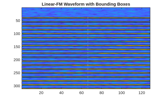

figure
imagesc(stftimtrain{4}(:,:,1))
for ii = 1:size(bboxestrain{4},1)
    drawrectangle(Position=bboxestrain{4}(ii,:),Color=[0 0 0],LineWidth=0.25,MarkerSize=0.01);
end
title("Rectangular-Pulse Waveform with Bounding Boxes")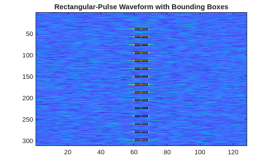

If you zoom in on the image for the rectangular-pulse spectrogram, it appears that the bounding box computation here may underestimate the actual bandwidth. The bandwidth for the rectangular pulses in this data were based on the reciprocal of the pulse width. In terms of accurately estimating the bandwidth for object detection, some other method may be preferable.

One important consideration to keep in mind with YOLO networks, is that the networks feature multiple convolutional layers with striding. This results in a significant reduction in the image size through the network. Additionally, there are pooling operations inside the network along the spatial dimensions. This can impact the estimation of bounding boxes, which are narrow in any of the [x,y,w,h] dimensions. This is a common case with radar waveforms where the time support can be especially small. In [2], the authors use a custom YOLO-like network where the padding on the convolutional layers is set to "same" to retain the size of the image. Fortunately, the yoloxObjectDetector used in this example allows you to specify image input sizes larger than the actual image along the two spatial dimensions. The images are automatically resized internally along with any bounding boxes. The detector automatically corrects the dimensions of these bounding boxes when the detect object function is used.

Training YOLOX on Max-pooled Spectrograms

If you wish to skip the training of the YOLOX detector, you can skip directly to the Evaluate Object Detector section. To set up the YOLOX detector for training, specify the input size to be 624-by-256-by-3. Here we increase the x- and y-dimensions of the image by a factor of 2. If you train your own model, you may even try a factor of 3 for the y-dimension of the image. As previously mentioned, the YOLOX network expects 3-channel images. Here we use the "small-coco" network. To learn more about the different network options, see yoloxObjectDetector (Computer Vision Toolbox). Here we denote the rectangular pulse class as "RP" and the linear FM waveform class as "FM".

inputSize = [2*312 2*128 3];
classes = ["RP" "FM"];
detector = yoloxObjectDetector("small-coco",classes,InputSize=inputSize);

For the training options, use a SGDM optimizer with a minibatch size of 20 and train for 30 epochs. We set the L2 regularization metric value to 0.1 and use the mAPObjectDetectionMetric metric to track the mean average precision (mAP) during training. Set the overlap threshold to be 0.3. Output the trained network with the best mean average precision metric. To train the network, set doTraining equal to true. Training with this data takes about 1 hour with a NVIDIA Titan V GPU with a compute capability of 7.0.

doTraining = false;
if doTraining
    options = trainingOptions("sgdm", ...
        InitialLearnRate=0.001, ...
        MiniBatchSize=20, ...
        MaxEpochs=30, ... 
        L2Regularization=0.1, ...
        Shuffle="once", ...
        Plots="training-progress", ...
        OutputNetwork= "best-validation", ...
        ResetInputNormalization = true, ...
        ValidationData= yolovalDS, ...
        Metrics=mAPObjectDetectionMetric(Name="mAP50",OverlapThreshold=0.3), ...
        ObjectiveMetricName="mAP50"); %#ok<*UNRCH>
    trainedRadarDetectorMAP30 = trainYOLOXObjectDetector(yolotrainDS,detector,options);
end

Evaluate Object Detector

If you did not train the object detector in the example, load the trained detector.

if ~doTraining 
    load(fullfile(datasetFolder,"testdata","trainedRadarDetectorMAP30.mat"));
end

Load the test data. The test data consists of 50 rectangular-pulse radar waveforms and 50 linear-FM waveforms.

load(fullfile(datasetFolder,"testdata","RPFMradardataTest.mat"));
load(fullfile(datasetFolder,"testdata","RPFMradardataTestLabels.mat"));
load(fullfile(datasetFolder,"testdata","RPFMradardataTestmetaData.mat"));

The helper function, createTestsetDS, repeats the earlier steps explicitly done for the training and validation sets and returns a CombinedDatastore for use in evaluating objector performance. The number of rectangular-pulsed waveform bounding boxes is returned in numPW and the number of linear-FM waveform bounding boxes is in numFM.

[yolotestDS,numRP,numFM] = createTestsetDS(RPFMradardataTest, ...
    RPFMradardataTestLabels,RPFMradardataTestmetaData,window=rectwin(16));
numRP

numRP = 
718

numFM

numFM = 
775

Note there are 718 rectangular-pulsed waveforms and 775 linear-FM waveform objects in the test set images. Evaluate the trained object detector on test images to measure the detector performance. The Computer Vision Toolbox™ provides an object detector evaluation function, evaluateObjectDetection, to measure common metrics such as average precision and precision-recall, with an option to specify the overlap thresholds at which to compute the metrics. Run the detector on the test data set using the detect object function. To evaluate the detector precision across the full range of recall values, set the detection threshold to a low value to detect as many objects as possible.

detectionThreshold = 0.001;
results = detect(trainedRadarDetectorMAP30,yolotestDS, ...
    MiniBatchSize=8,Threshold=detectionThreshold);

Compute Metrics at Specified Overlap Thresholds

Compute the object detection metrics at specified overlap thresholds using the evaluateObjectDetection function. The overlap threshold defines the fraction of amount of overlap required between a predicted bounding box and a ground truth bounding box for the predicted bounding box to count as a true positive. For example, an overlap threshold of 0.5 considers an overlap of 50% between boxes as a correct match, while an overlap threshold of 0.9 is stricter and requires the predicted bounding box to almost exactly coincide with the ground truth bounding box. Specify five overlap thresholds at which to compute metrics using the overlapThresholds variable.

overlapThresholds = [0.3 0.4 0.5 0.75 0.9];
metrics = evaluateObjectDetection(results,yolotestDS,overlapThresholds);

Evaluate Object Detection Metrics Summary

Evaluate the summarized detector performance at the overall dataset level and at the individual class level using the summarize object function.

[datasetSummary,classSummary] = summarize(metrics)

datasetSummary=1×7 table
    NumObjects    mAPOverlapAvg    mAP0.3     mAP0.4     mAP0.5     mAP0.75       mAP0.9  
    __________    _____________    _______    _______    _______    ________    __________

       1493          0.59715       0.99999    0.99024    0.90373    0.091801    4.1451e-06

classSummary=2×7 table
          NumObjects    APOverlapAvg     AP0.3      AP0.4      AP0.5      AP0.75       AP0.9   
          __________    ____________    _______    _______    _______    ________    __________

    RP       718          0.56599             1    0.98178    0.81003    0.038126    8.2902e-06
    FM       775          0.62832       0.99998     0.9987    0.99742     0.14548             0

By default, the summarize object function returns summarized data set and class metrics at all overlap thresholds. Detections with a higher IoU value correspond to a lower average precision (AP) or mean average precision (mAP) value. The AP metric provides a single number that incorporates the ability of the detector to make correct classifications (precision) and the ability of the detector to find all relevant objects (recall). The mAP is the average of the AP calculated for all the classes. To evaluate the detector performance at the data set level, consider the mAP averaged over all overlap thresholds, returned in the mAPOverlapAvg column of the datasetSummary output. At the overlap threshold of 0.5, the mAP is approximately 0.90, which indicates that the detector is able to find most objects without making too many spurious predictions. At higher overlap thresholds, such as 0.75 and 0.9, the mAP is significantly lower since the matching condition between predicted and ground truth boxes is now much stricter. Similarly, to evaluate the detector performance at the class level, consider the AP averaged over all IoU thresholds, returned in the APOverlapAvg column of the classSummary output.

Overall, the summary shows that the object detector performed well on the held-out test set. Subsequent sections use these metrics to select the best confidence score and overlap threshold for this test set.

Choose Threshold based on Best F1 Score

To choose the best confidence score threshold for the held-out test, use the precision and recall values for each class to determine the best F1 score as a function of object confidence score. Determine the object confidence score threshold as the value at which the F1 score maximum occurs across the two classes. The F1 score is the harmonic mean of the precision and recall values. Determine those as a function of confidence score for both the rectangular-pulsed and linear-FM waveforms.

[precisionRP,recallRP,scoresRP] = precisionRecall(metrics,ClassName="RP");
[precisionFM,recallFM,scoresFM] = precisionRecall(metrics,ClassName="RP");
f1scoresRP = cellfun(@harmmean,cellfun(@(x,y)cat(1,x,y),precisionRP,recallRP,uniform=false),uniform=false);
f1scoresRP = cell2mat(f1scoresRP')';
f1scoresFM = cellfun(@harmmean,cellfun(@(x,y)cat(1,x,y),precisionFM,recallFM,uniform=false),uniform=false);
f1scoresFM = cell2mat(f1scoresFM')';

Because the detector is clearly performing the best for overlap thresholds of 0.3, 0.4, and 0.5, plot the F1 scores for those thresholds as a function of the confidence score.

tiledlayout(2,1)
ax1 = nexttile;
plot(scoresRP{:},f1scoresRP(:,1:3))
grid on
title(classes(1) + " F1-Scores"); 
legend(string(overlapThresholds(1:3)) + " IoU",Location="bestoutside")
ax2 = nexttile;
plot(scoresFM{:},f1scoresFM(:,1:3))
grid on
title(classes(2) + " F1-Scores"); 
legend(string(overlapThresholds(1:3)) + " IoU",Location="bestoutside")

For both classes there is essentially no difference between the F1 scores for IoU thresholds of 0.3 and 0.4. Also, note that for both classes the F1 scores are near their maximum values over a range of 0.1 to 0.4.

Evaluate Detector Errors Using Confusion Matrix

The confusion matrix enables you to quantify how well the object detector performs across different classes by providing a detailed breakdown of the detection errors. Investigate the types of classification errors made by the detector at a selected confidence level and overlap threshold by using the confusionMatrix object function. Based on the analysis of the F1 scores by confidence score and overlap threshold, use a confidence score of 0.4 and an overlap threshold of 0.4 to evaluate the model on the held-out test set.

OT = overlapThresholds(2);
detectionThresh = 0.4;
[confMat,confusionClassNames] = confusionMatrix(metrics,scoreThreshold=detectionThresh,overlapThreshold=OT);
figure
confusionchart(confMat{1},confusionClassNames)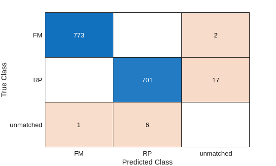

The confusion chart shows that the detector has detected approximately 99% of the linear-FM waveforms with a confidence score of at least 0.4. For the rectangular-pulse waveforms, the detector has correctly identified the pulse type and time-frequency bounding box in approximately 97% of the waveforms. The detector missed 17 of the rectangular-pulsed waveforms, while missing 2 linear-FM pulses. The network made 6 false predictions of rectangular pulses and 1 false prediction of a linear-FM pulse. Note that if you train the network yourself, results may differ slightly.

Radar Parameter Estimation and Noise-Only Signals

This section shows how to apply the trained detector to a couple of the held-out test images and use the outputs to estimate the radar parameters. You may find it useful to consult YOLO-like Object Detection in Radar for how to interpret the outputs of the detect (Computer Vision Toolbox) object function. First, read all the test data and obtain the estimates for a rectangular-pulse waveform.

testdata = readall(yolotestDS);
[bboxestestRP,scorestestRP,labelstestRP,infotestRP] = detect(trainedRadarDetectorMAP30,testdata{1,1});

Looking at the outputs of the detect function, there are 14 bounding boxes (bboxestestRP) detected corresponding to 14 objects in the spectrogram. The output, scorestestRP, contains the products of the class probabilities and the object confidence scores referenced in YOLO-like Object Detection in Radar. labelstestRP contains the class labels for the detected pulses. infotestRP is a structure array containing two fields, ClassProbabilities and ObjectnessScore. Recall that one output of YOLOX is the class probability. Because there are two classes in this data, there is a probability for each class and each bounding box.

infotestRP.ClassProbabilities

ans = 14×2 single matrix

    0.6707    0.0011
    0.6541    0.0010
    0.6837    0.0009
    0.6487    0.0006
    0.6702    0.0009
    0.6575    0.0006
    0.6551    0.0006
    0.6796    0.0009
    0.6590    0.0009
    0.6341    0.0009
    0.6839    0.0008
    0.6204    0.0009
    0.6687    0.0009
    0.6225    0.0009
      ⋮

If you take these probabilities and multiply them by the ObjectnessScore, you obtain the overall confidence score for each object. Compare the bounding boxes returned by the detector with the ground-truth estimates for the test signal. Package the estimates in a table for readability.

estboxesandGTRP = [bboxestestRP(:,1) testdata{1,2}(:,1) bboxestestRP(:,2) ...
    testdata{1,2}(:,2) bboxestestRP(:,3) testdata{1,2}(:,3) bboxestestRP(:,4) testdata{1,2}(:,4)];
bboxtblcompareRP = array2table(estboxesandGTRP,VariableNames = ["XEstimate" "XTruth" "YEstimate" ... 
        "YTruth" "WEstimate" "WTruth" "HEstimate" "HTruth"])

bboxtblcompareRP=14×8 table
    XEstimate    XTruth    YEstimate    YTruth    WEstimate    WTruth    HEstimate    HTruth
    _________    ______    _________    ______    _________    ______    _________    ______

     59.561      58.429      39.15      38.561     11.181      12.143     3.0349      3.0273
     59.357      58.429     59.362      58.696     11.708      12.143     3.0966      3.0273
     58.961      58.429     79.627      78.831     12.368      12.143     3.0687      3.0273
     58.193      58.429     99.551      98.966     13.687      12.143     3.1164      3.0273
     58.267      58.429     119.64       119.1     13.558      12.143     3.1298      3.0273
     57.898      58.429     139.57      139.24     14.313      12.143     3.0793      3.0273
     58.032      58.429     159.56      159.37     14.038      12.143     3.1014      3.0273
     58.488      58.429     180.26      179.51     13.351      12.143     3.0932      3.0273
     59.328      58.429     200.29      199.64     11.736      12.143     3.0843      3.0273
     59.575      58.429     220.36      219.78     11.402      12.143     3.1221      3.0273
      59.93      58.429     240.31      239.91     10.403      12.143     3.0559      3.0273
     60.015      58.429     260.29      260.05     10.363      12.143     3.1364      3.0273
     59.416      58.429     280.26      280.18     11.265      12.143     3.0701      3.0273
     60.228      58.429     300.19      300.32     10.113      12.143     3.1192      3.0273

The above units are in pixels based on the input image. Note the ground-truth values for the h-coordinate are slightly larger than 3. As previously mentioned, this was done to mitigate the effect that the actual pulse duration is often less than 1 pixel. If you subtract 3 from the HTruth values, you see they equal 0.0273 which in the time units of the max-pooled spectrogram is equal to 0.0273*51.2e-6 = 1.3978e-06, which is essentially equal to RPFMradardataTestmetaData{1,"PulseWidth"}. For the bandwidth measurements, keep in mind those are in units of the DFT bin spacing which is 1e7/128 in this example. Compare the bandwidth estimates (w-coordinate) against the ground truth using the information about the spacing of the DFT bins to convert from pixels to Hz.

dftspacing = 1e7/128;
pixelBuffer = 3;
array2table([(bboxtblcompareRP.WEstimate-pixelBuffer)*(1e7/128) (bboxtblcompareRP.WTruth-pixelBuffer)*(1e7/128)], ...
    VariableNames=["Estimated BW (Hz)" "Ground Truth BW (Hz)"])

ans=14×2 table
    Estimated BW (Hz)    Ground Truth BW (Hz)
    _________________    ____________________

       6.3914e+05             7.1429e+05     
        6.803e+05             7.1429e+05     
       7.3188e+05             7.1429e+05     
       8.3492e+05             7.1429e+05     
       8.2486e+05             7.1429e+05     
       8.8384e+05             7.1429e+05     
       8.6231e+05             7.1429e+05     
       8.0869e+05             7.1429e+05     
       6.8252e+05             7.1429e+05     
       6.5641e+05             7.1429e+05     
       5.7839e+05             7.1429e+05     
       5.7527e+05             7.1429e+05     
       6.4574e+05             7.1429e+05     
       5.5573e+05             7.1429e+05     

The estimated BWs are quite close to the ground truth. Finally, compare the estimated start times of the pulses in YEstimate against the ground truth. Recall that the pulses always begin at 0.002 seconds.

timeSlotFactor = 32*16*1e-7;
array2table([bboxtblcompareRP.YEstimate.*timeSlotFactor bboxtblcompareRP.YTruth.*timeSlotFactor], ...
        VariableNames=["Estimated Pulse STart (seconds)" "Ground Truth Pulse Start (seconds)"])

ans=14×2 table
    Estimated Pulse STart (seconds)    Ground Truth Pulse Start (seconds)
    _______________________________    __________________________________

               0.0020045                           0.0019743             
               0.0030393                           0.0030052             
               0.0040769                           0.0040362             
                0.005097                           0.0050671             
               0.0061256                            0.006098             
               0.0071459                           0.0071289             
               0.0081696                           0.0081599             
               0.0092292                           0.0091908             
                0.010255                            0.010222             
                0.011282                            0.011253             
                0.012304                            0.012284             
                0.013327                            0.013315             
                0.014349                            0.014345             
                 0.01537                            0.015376             

The estimated pulse start times are in good agreement with the ground truth.

Compare the ground-truth and estimated bounding boxes for a linear-FM waveform.

[bboxestestFM,scorestestFM,labelstestFM,infotestFM] = detect(trainedRadarDetectorMAP30,testdata{5,1});
estboxesandGTFM = [bboxestestFM(:,1) testdata{5,2}(:,1) bboxestestFM(:,2) ...
    testdata{5,2}(:,2) bboxestestFM(:,3) testdata{5,2}(:,3) bboxestestFM(:,4) testdata{5,2}(:,4)];
bboxtblcompareFM = array2table(estboxesandGTFM,VariableNames = ["XEstimate" "XTruth" "YEstimate" ... 
        "YTruth" "WEstimate" "WTruth" "HEstimate" "HTruth"])

bboxtblcompareFM=22×8 table
    XEstimate    XTruth    YEstimate    YTruth    WEstimate    WTruth    HEstimate    HTruth
    _________    ______    _________    ______    _________    ______    _________    ______

     7.2861        1        38.911      38.561     119.88       131       3.3901      4.1719
      5.251        1        48.528      48.326     122.75       131       3.3345      4.1719
     7.0552        1        58.352      58.092      120.3       131       3.3833      4.1719
      4.629        1        68.198      67.857     123.37       131       3.4125      4.1719
     6.6548        1        78.192      77.623     120.72       131       3.4654      4.1719
     5.8406        1         87.62      87.389     122.16       131        3.486      4.1719
     5.4692        1        97.551      97.154     122.53       131        3.324      4.1719
     7.3019        1        107.23      106.92     119.49       131       3.4176      4.1719
      4.159        1        117.04      116.69     123.84       131       3.4349      4.1719
     7.8007        1         126.6      126.45     118.49       131       3.4171      4.1719
      5.321        1        136.31      136.22     122.68       131       3.3768      4.1719
     7.3019        1        146.43      145.98     119.67       131       3.3835      4.1719
     4.8929        1        156.13      155.75     123.11       131       3.4259      4.1719
     4.4123        1        165.91      165.51     123.59       131       3.6028      4.1719
     6.2084        1        175.22      175.28     121.79       131        3.471      4.1719
      4.027        1        185.24      185.04     123.97       131       3.4748      4.1719
      ⋮

Again, the agreement is quite good in this case, except for the x-estimate which is the starting frequency in Hz.

Even though the YOLOX network in this example was not trained with examples of noise-only spectrograms, YOLOX looks at the entire image during training to detect objects and estimate their locations and size. This means that the network is explicitly exposed to noise-only regions as long as the image has sufficient areas where there are no objects. Because those areas were present in these spectrograms, we did not include noise-only samples in the training data. The following code loads three signals consisting of just complex-valued white Gaussian noise. The noise was generated in the same manner as the additive noise present in the training and test data. Load the noise-only signals and obtain the max-pooled spectrograms. Because the YOLOX detector expects 3-channel images, replicate the spectrogram in each channel. Run the detector on the generated images.

load('noiseOnlyTest.mat')
S1 = maxpooledSTFT(noiseOnlyTest(:,1),128,32,rectwin(16));
S1 = repmat(S1,1,1,3);
[bboxes1,~,labels1] = detect(trainedRadarDetectorMAP30,S1,Threshold=detectionThresh)

bboxes1 =

  0×4 empty single matrix


labels1 = 

  0×1 empty categorical array

S2 = maxpooledSTFT(noiseOnlyTest(:,2),128,32,rectwin(16));
S2 = repmat(S2,1,1,3);
[bboxes2,~,labels2] = detect(trainedRadarDetectorMAP30,S2,Threshold=detectionThresh)

bboxes2 =

  0×4 empty single matrix


labels2 = 

  0×1 empty categorical array

S3 = maxpooledSTFT(noiseOnlyTest(:,3),128,32,rectwin(16));
S3 = repmat(S3,1,1,3);
[bboxes3,~,labels3] = detect(trainedRadarDetectorMAP30,S3,Threshold=detectionThresh)

bboxes3 =

  0×4 empty single matrix


labels3 = 

  0×1 empty categorical array

The detector finds no radar objects in the data as evidenced by the empty bounding boxes and labels. This demonstrates that even though the YOLOX network has not been trained explicitly on noise-only spectrograms, the network has seen enough areas of the time-frequency representation devoid of radar pulses to learn when no object is present. Of course, you can elect to include noise-only images in your training and in certain situations that may be even be beneficial to training a robust detector.

Summary

This example shows how to set up and train a YOLOX object detector on pooled spectrograms of rectangular-pulsed and linear-FM pulse waveforms. YOLO-like detectors have the potential to perform well on identifying radar waveforms and estimating their parameters over a range of pulse parameters and SNRs. In this case, the YOLOX detector did an impressive job of correctly classifying the two pulse types with a range of parameterizations as well as correctly identifying the time-frequency extent of the pulse. The method used in this example for determining the ground-truth bounding boxes may not be optimal. For example, you may have more precise calculations for your data to rely on, or you can use Image Labeler (Computer Vision Toolbox) to create bounding boxes for your training data, which may be more accurate in many cases.

Detections were also greatly aided by the use of the max-pooled spectrogram introduced in [2]. While the range of SNRs used in this example (17-20 dB) were on the high end of those typically encountered in realistic radar scenarios, this example demonstrates that the YOLOX detector shows promise in reliably detecting small objects representing radar pulses in the time-frequency plane.

References

[1] Caromi, Raied, Michael Souryal, and Timothy A. Hall. "RF Dataset of Incumbent Radar Signals in the 3.5GHz CBRS Band." Journal of Research of the National Institute of Standards and Technology 124 (December 17, 2017). https://doi.org/10.6028/jres.124.038.

[2] Sarkar, Shamik, Dongning Guo, and Danijela Cabric. "Radyololet: Radar Detection and Parameter Estimation using Yolo and Wavelet." IEEE Transactions on Cognitive Communications and Networking, 2024, 1-1. https://doi.org/10.1109/tccn.2024.3519315.