Node Classification Using Graph Convolutional Network
This example shows how to classify nodes in a graph using a graph convolutional network (GCN).
To predict categorical labels of the nodes in a graph, you can use a GCN [1]. For example, you can use a GCN to predict types of atoms in a molecule (for example, carbon and oxygen) given the molecular structure (the chemical bonds represented as a graph).
A GCN is a variant of a convolutional neural network that takes two inputs:
An -by- feature matrix , where is the number of nodes of the graph and is the number channels per node.
An -by- adjacency matrix that represents the connections between nodes in the graph.
This figure shows some example node classifications of a graph.

Because the graph data is sparse, a custom training loop is best suited for training a GCN. This example shows how to train a GCN using a custom training loop with the QM7 dataset [2] [3], which is a molecular data set consisting of 7165 molecules composed of up to 23 atoms. That is, the molecule with the highest number of atoms has 23 atoms.
Download and Load QM7 Data
Download the QM7 data set from the https://quantum-machine.org/data/qm7.mat. The data set consists of five unique atoms: carbon, hydrogen, nitrogen, oxygen, and sulphur.
dataURL = "https://quantum-machine.org/data/qm7.mat";
outputFolder = fullfile(tempdir,"qm7Data");
dataFile = fullfile(outputFolder,"qm7.mat");

if ~exist(dataFile,"file")
    mkdir(outputFolder);
    disp("Downloading QM7 data...");
    websave(dataFile, dataURL);
    disp("Done.")
end
The MAT file contains consists of five different arrays. This example uses the arrays X and Z, which represent the Coulomb matrix [3] representation of each molecule and the atomic numbers of each atom of the molecule, respectively. Molecules in the data that have fewer than 23 atoms are padded with zeros.
Load the QM7 data from the MAT file.
data = load(dataFile)
data = struct with fields:
    X: [7165×23×23 single]
    R: [7165×23×3 single]
    Z: [7165×23 single]
    T: [-417.9600 -712.4200 -564.2100 -404.8800 -808.8700 -677.1600 -796.9800 -860.3300 -1.0085e+03 -861.7300 -708.3700 -725.9300 -879.3800 -618.7200 -871.1900 -653.4400 -1.0109e+03 -1.1594e+03 -1.0039e+03 -1.0184e+03 -1.0250e+03 -1.1750e+03 … ]
    P: [5×1433 int64]
Extract the Coulomb data and the atomic numbers from the loaded structure. Permute the Coulomb data so that the third dimension corresponds to the observations. Sort the atomic numbers in descending order.
coulombData = double(permute(data.X, [2 3 1]));
atomData = sort(data.Z,2,'descend');
View the atoms of the first observation. The number of nonzero elements indicates the number of different atoms in the molecule. Each nonzero element corresponds to the atomic number of a specific element in the molecule.
atomData(1,:)
ans = 1×23 single row vector

     6     1     1     1     1     0     0     0     0     0     0     0     0     0     0     0     0     0     0     0     0     0     0
Preprocess Graph Data
The GCN used in this example requires the Coulomb matrices as feature input as well as the corresponding adjacency matrices.
To convert the Coulomb matrices in the training data to adjacency matrices, use the coulomb2Adjacency function, attached to this example as a supporting file. To access this file, open the example as a live script. To facilitate splitting the data into separate molecules for training, validation, and inference, the coloumb2Adjacency function does not remove padded zeros from the data.
adjacencyData = coulomb2Adjacency(coulombData,atomData);
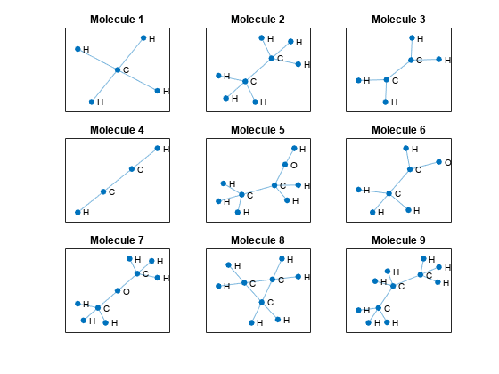
Visualize the first few molecules in a plot. For each molecule, extract the unpadded adjacency matrix and plot the graph with labeled nodes. To convert atomic numbers to symbols, use the atomicSymbol function, attached to this example as a supporting file. To access this function, open the example as a live script.
figure
tiledlayout("flow")

for i = 1:9
    % Extract unpadded adjacency matrix.
    atomicNumbers = nonzeros(atomData(i,:));
    numNodes = numel(atomicNumbers);
    A = adjacencyData(1:numNodes,1:numNodes,i);

    % Convert adjacency matrix to graph.
    G = graph(A);

    % Convert atomic numbers to symbols.
    symbols = atomicSymbol(atomicNumbers);

    % Plot graph.
    nexttile
    plot(G,NodeLabel=symbols,Layout="force")
    title("Molecule " + i)
end

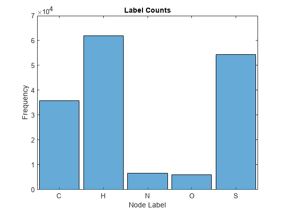
Visualize the frequency of each label category using a histogram.
figure
histogram(categorical(atomicSymbol(atomData)))
xlabel("Node Label")
ylabel("Frequency")
title("Label Counts")

Partition the data into training, validation, and test partitions containing 80%, 10%, and 10% of the data, respectively. To get a random split, use the trainingPartitions function, attached to this example as a supporting file. To access this file, open the example as a live script.
numObservations = size(adjacencyData,3);
[idxTrain,idxValidation,idxTest] = trainingPartitions(numObservations,[0.8 0.1 0.1]);

adjacencyDataTrain = adjacencyData(:,:,idxTrain);
adjacencyDataValidation = adjacencyData(:,:,idxValidation);
adjacencyDataTest = adjacencyData(:,:,idxTest);

coulombDataTrain = coulombData(:,:,idxTrain);
coulombDataValidation = coulombData(:,:,idxValidation);
coulombDataTest = coulombData(:,:,idxTest);

atomDataTrain = atomData(idxTrain,:);
atomDataValidation = atomData(idxValidation,:);
atomDataTest = atomData(idxTest,:);
Preprocess the training and validation data using the preprocessData function, defined in the Preprocess Data Function section of the example. The preprocessData function builds a sparse block-diagonal matrix of the adjacency matrices of different graph instances such that each block in the matrix corresponds to the adjacency matrix of one graph instance. This preprocessing is required because a GCN accepts a single adjacency matrix as input, whereas this example deals with multiple graph instances. The function takes the nonzero diagonal elements of the Coulomb matrices and assigns them as features. Therefore, the number of input features per node in the example is 1.
[ATrain,XTrain,labelsTrain] = preprocessData(adjacencyDataTrain,coulombDataTrain,atomDataTrain);
size(XTrain)
ans = 1×2

       88424           1
size(labelsTrain)
ans = 1×2

       88424           1
[AValidation,XValidation,labelsValidation] = preprocessData(adjacencyDataValidation,coulombDataValidation,atomDataValidation);
Normalize the features using the mean and variance of the training features. Normalize the validation features using the same statistics.
muX = mean(XTrain);
sigsqX = var(XTrain,1);

XTrain = (XTrain - muX)./sqrt(sigsqX);
XValidation = (XValidation - muX)./sqrt(sigsqX);
Define Deep Learning Model
Define the following deep learning model, which takes as input an adjacency matrix and a feature matrix and outputs categorical predictions.

The multiplication operations are weighted multiplication operations with learnable weights.
In more detail, the model is a series of operations of the form (the final operation does not include the addition step). In this formula:
is the activation function.
.
is the weight matrix for the multiplication.
is the adjacency matrix of graph with added self-connections. is the identity matrix.
is the degree matrix of .
The expression is also known as the normalized adjacency matrix of the graph.
Initialize Model Parameters
Define the parameters for each of the operations and include them in a structure. Use the format parameters.OperationName.ParameterName where parameters is the structure, OperationName is the name of the operation (for example, multiply1), and ParameterName is the name of the parameter (for example, Weights).
Create a structure parameters containing the model parameters.
parameters = struct;
Initialize the learnable weights using the initializeGlorot function, attached to this example as a supporting file. To access this function, open the example as a live script.
Initialize the weights of the first multiply operation. Initialize the weights to have an output size of 32. The input size is the number of channels of the input feature data.
numHiddenFeatureMaps = 32;
numInputFeatures = size(XTrain,2);

sz = [numInputFeatures numHiddenFeatureMaps];
numOut = numHiddenFeatureMaps;
numIn = numInputFeatures;
parameters.mult1.Weights = initializeGlorot(sz,numOut,numIn,"double");
Initialize the weights of the second multiply operation. Initialize the weights to have the same output size as the previous multiply operation. The input size is the output size of the previous multiply operation.
sz = [numHiddenFeatureMaps numHiddenFeatureMaps];
numOut = numHiddenFeatureMaps;
numIn = numHiddenFeatureMaps;
parameters.mult2.Weights = initializeGlorot(sz,numOut,numIn,"double");
Initialize the weights of the third multiply operation. Initialize the weights to have an output size matching the number of classes. The input size is the output size of the previous multiply operation.
classes = categories(labelsTrain);
numClasses = numel(classes);

sz = [numHiddenFeatureMaps numClasses];
numOut = numClasses;
numIn = numHiddenFeatureMaps;
parameters.mult3.Weights = initializeGlorot(sz,numOut,numIn,"double");
View the parameters structure.
parameters
parameters = struct with fields:
    mult1: [1×1 struct]
    mult2: [1×1 struct]
    mult3: [1×1 struct]
View the parameters of the first multiply operation.
parameters.mult1
ans = struct with fields:
    Weights: [1×32 dlarray]
Define Model Function
Create the function model, defined in the Model Function section of the example, which takes as input the model parameters, the feature data, and the adjacency matrix, and returns the predictions.
Define Model Loss Function
Create the function modelLoss, defined in the Model Loss Function section of the example, which takes as input the model parameters, the feature data, the adjacency matrix, and the one-hot encoded targets, and returns the loss, the gradients of the loss with respect to the parameters, and the network predictions.
Specify Training Options
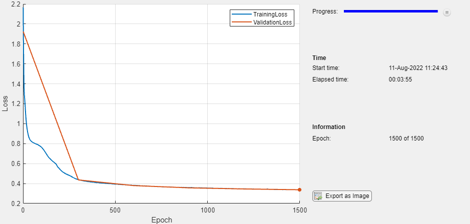
Train for 1500 epochs and set the learning rate for the Adam solver to 0.01.
numEpochs = 1500;
learnRate = 0.01;
Validate the network after every 300 epochs.
validationFrequency = 300;
Train Model
Initialize parameters for Adam.
trailingAvg = [];
trailingAvgSq = [];
Convert the training and validation feature data to dlarray objects.
XTrain = dlarray(XTrain);
XValidation = dlarray(XValidation);
Train on a GPU if one is available. Using a GPU requires Parallel Computing Toolbox™ and a supported GPU device. For information on supported devices, see GPU Computing Requirements (Parallel Computing Toolbox) (Parallel Computing Toolbox). To train on a GPU, convert the data to gpuArray objects.
if canUseGPU
    XTrain = gpuArray(XTrain);
end
Convert the training and validation labels to one-hot encoded vectors using the onehotencode function.
TTrain = onehotencode(labelsTrain,2,ClassNames=classes);
TValidation = onehotencode(labelsValidation,2,ClassNames=classes);
Initialize the TrainingProgressMonitor object.
monitor = trainingProgressMonitor( ...
    Metrics=["TrainingLoss","ValidationLoss"], ...
    Info="Epoch", ...
    XLabel="Epoch");

groupSubPlot(monitor,"Loss",["TrainingLoss","ValidationLoss"])
Train the model using a custom training loop. The training uses full-batch gradient descent.
For each epoch:
Evaluate the model loss and gradients using
dlfevaland themodelLossfunction.Update the network parameters using
adamupdate.Update the training plot.
If required, validate the network by making predictions using the
modelfunction and plotting the validation loss.
epoch = 0;

while epoch < numEpochs && ~monitor.Stop
    epoch = epoch + 1;

    % Evaluate the model loss and gradients.
    [loss,gradients] = dlfeval(@modelLoss,parameters,XTrain,ATrain,TTrain);

    % Update the network parameters using the Adam optimizer.
    [parameters,trailingAvg,trailingAvgSq] = adamupdate(parameters,gradients, ...
        trailingAvg,trailingAvgSq,epoch,learnRate);

    % Record the training loss and epoch.
    recordMetrics(monitor,epoch,TrainingLoss=loss);
    updateInfo(monitor,Epoch=(epoch+" of "+numEpochs));

    % Display the validation metrics.
    if epoch == 1 || mod(epoch,validationFrequency) == 0
        YValidation = model(parameters,XValidation,AValidation);
        lossValidation = crossentropy(YValidation,TValidation,DataFormat="BC");

        % Record the validation loss.
        recordMetrics(monitor,epoch,ValidationLoss=lossValidation);
    end

    monitor.Progress = 100*(epoch/numEpochs);
end

Test Model
Test the model using the test data.
Preprocess the test data using the same steps as for the training and validation data.
[ATest,XTest,labelsTest] = preprocessData(adjacencyDataTest,coulombDataTest,atomDataTest);
XTest = (XTest - muX)./sqrt(sigsqX);
Convert the test feature data to a dlarray object.
XTest = dlarray(XTest);
Make predictions on the data and convert the probabilities to categorical labels using the onehotdecode function.
YTest = model(parameters,XTest,ATest);
YTest = onehotdecode(YTest,classes,2);
Calculate the accuracy.
accuracy = mean(YTest == labelsTest)
accuracy = 0.8930
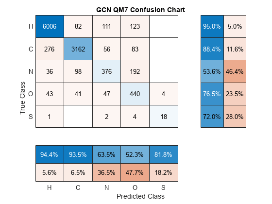
To visualize how the model makes incorrect predictions and evaluate the model based on class-wise precision and class-wise recall, calculate the confusion matrix using the confusionchart function.
The per-class precision is the ratio of true positives to total positive predictions for a class. The total positive predictions include the true positives and false positives. A false positive is an outcome where the model incorrectly predicts a class as present in an observation. The per-class recall, also known as true positive rate, is the ratio of true positives to total positive observations for a class. The total positive observation includes the true positives and false negatives. A false negative is an outcome where the model incorrectly predicts a class as absent in an observation.
figure
cm = confusionchart(labelsTest,YTest, ...
    ColumnSummary="column-normalized", ...
    RowSummary="row-normalized");
title("GCN QM7 Confusion Chart");

The per-class precision scores are in the first row of the column summary of the chart and the per-class recall scores are in the first column of the row summary of the chart.
Predict Using New Data
Make some predictions on unlabeled data using the modelPredictions function, listed in the Model Predictions Function section of the example. For simplicity, use the first few observations of the test data.
numObservationsNew = 4;
adjacencyDataNew = adjacencyDataTest(:,:,1:numObservationsNew);
coulombDataNew = coulombDataTest(:,:,1:numObservationsNew);

predictions = modelPredictions(parameters,coulombDataNew,adjacencyDataNew,muX,sigsqX,classes);
Visualize the predictions in a plot. For each molecule, create the graph representation using the adjacency matrix and label the nodes with the predictions.
figure
tiledlayout("flow")

for i = 1:numObservationsNew
    % Extract unpadded adjacency data.
    numNodes = find(any(adjacencyDataTest(:,:,i)),1,"last");

    A = adjacencyDataTest(1:numNodes,1:numNodes,i);

    % Create and plot graph representation.
    nexttile
    G = graph(A);
    plot(G,NodeLabel=string(predictions{i}),Layout="force")
    title("Observation " + i + " Prediction")
end

Supporting Functions
Preprocess Data Function
The preprocessData function preprocesses the adjacency, Coulomb, and atom data using the following steps:
Preprocess the adjacency and Coulomb matrices using the
preprocessPredictorsfunction, listed in the Preprocess Predictors Function section of the example.Convert the atom data to a flattened array of categorical labels.
function [adjacency,features,labels] = preprocessData(adjacencyData,coulombData,atomData)

[adjacency, features] = preprocessPredictors(adjacencyData,coulombData);
labels = [];

% Convert labels to categorical.
for i = 1:size(adjacencyData,3)
    % Extract and append unpadded data.
    T = nonzeros(atomData(i,:));
    labels = [labels; T];
end

labels2 = nonzeros(atomData);
assert(isequal(labels2,labels2))

atomicNumbers = unique(labels);
atomNames =  atomicSymbol(atomicNumbers);
labels = categorical(labels, atomicNumbers, atomNames);

end
Preprocess Predictors Function
The preprocessPredictors function preprocesses the adjacency and Coulomb matrices using the following steps:
For each molecule:
Extract the unpadded data.
Extract the feature vector from the diagonal of the unpadded Coulomb matrix.
Append the extracted data to the output arrays.
For the adjacency matrix input, the GCN requires a single sparse block-diagonal matrix containing each of the adjacency matrices, where each block corresponds to the adjacency matrix of one graph instance. To append data to the block-diagonal matrix, the function uses the blkdiag function.
function [adjacency,features] = preprocessPredictors(adjacencyData,coulombData)

adjacency = sparse([]);
features = [];

for i = 1:size(adjacencyData, 3)
    % Extract unpadded data.
    numNodes = find(any(adjacencyData(:,:,i)),1,"last");

    A = adjacencyData(1:numNodes,1:numNodes,i);
    X = coulombData(1:numNodes,1:numNodes,i);

    % Extract feature vector from diagonal of Coulomb matrix.
    X = diag(X);

    % Append extracted data.
    adjacency = blkdiag(adjacency,A);
    features = [features; X];
end

end
Model Function
The model function takes as input the model parameters parameters, the feature matrix X, and the adjacency matrix A, and returns the network predictions. In a preprocessing step, the model function calculates the normalized adjacency matrix using the normalizeAdjacency function, listed in the Normalize Adjacency Function section of the example. The normalized adjacency matrix corresponds to in the formula below.
The deep learning model takes as input an adjacency matrix and a feature matrix and outputs categorical predictions.

The multiplication operations are weighted multiply operations with learnable weights.
In more detail, the model is a series of operations of the form (the final operation does not include the addition step). In this formula:
is the activation function.
.
is the weight matrix for the multiplication.
is the adjacency matrix of graph with added self-connections. is the identity matrix.
is the degree matrix of .
function Y = model(parameters,X,A)

ANorm = normalizeAdjacency(A);

Z1 = X;

Z2 = ANorm * Z1 * parameters.mult1.Weights;
Z2 = relu(Z2) + Z1;

Z3 = ANorm * Z2 * parameters.mult2.Weights;
Z3 = relu(Z3) + Z2;

Z4 = ANorm * Z3 * parameters.mult3.Weights;
Y = softmax(Z4,DataFormat="BC");

end
Model Loss Function
The modelLoss function takes as input the model parameters parameters, the feature matrix X, the adjacency matrix A, and the one-hot encoded target data T, and returns the loss and the gradients of the loss with respect to the model parameters.
function [loss,gradients] = modelLoss(parameters,X,A,T)

Y = model(parameters,X,A);
loss = crossentropy(Y,T,DataFormat="BC");
gradients = dlgradient(loss, parameters);

end
Model Predictions Function
The modelPredictions function takes as input the model parameters, the input Coulomb and adjacency data, the normalization statistics mu and sigsq, and a list of the class names, and returns a cell array of the predicted node labels of the input data. The function makes predictions by looping over the input graphs one at a time.
function predictions = modelPredictions(parameters,coulombData,adjacencyData,mu,sigsq,classes)

predictions = {};
numObservations = size(coulombData,3);

for i = 1:numObservations
    % Extract unpadded data.
    numNodes = find(any(adjacencyData(:,:,i)),1,"last");
    A = adjacencyData(1:numNodes,1:numNodes,i);
    X = coulombData(1:numNodes,1:numNodes,i);

    % Preprocess data.
    [A,X] = preprocessPredictors(A,X);
    X = (X - mu)./sqrt(sigsq);
    X = dlarray(X);

    % Make predictions.
    Y = model(parameters,X,A);
    Y = onehotdecode(Y,classes,2);
    predictions{end+1} = Y;
end

end
Normalize Adjacency Function
The normalizeAdjacency function takes as input the adjacency matrix and returns the normalized adjacency matrix , where is the adjacency matrix of a graph with added self-connections, is the identity matrix, and is the degree matrix of .
function ANorm = normalizeAdjacency(A)

% Add self connections to adjacency matrix.
A = A + speye(size(A));

% Compute inverse square root of degree.
degree = sum(A, 2);
degreeInvSqrt = sparse(sqrt(1./degree));

% Normalize adjacency matrix.
ANorm = diag(degreeInvSqrt) * A * diag(degreeInvSqrt);

end
References
Kipf, Thomas N., and Max Welling. “Semi-Supervised Classification with Graph Convolutional Networks.” Paper presented at ICLR 2017, Toulon, France, April 2017.
Blum, Lorenz C., and Jean-Louis Reymond. “970 Million Druglike Small Molecules for Virtual Screening in the Chemical Universe Database GDB-13.” Journal of the American Chemical Society 131, no. 25 (July 1, 2009): 8732–33. https://doi.org/10.1021/ja902302h.
Rupp, Matthias, Alexandre Tkatchenko, Klaus-Robert Müller, and O. Anatole von Lilienfeld. “Fast and Accurate Modeling of Molecular Atomization Energies with Machine Learning.” Physical Review Letters 108, no. 5 (January 31, 2012): 058301. https://doi.org/10.1103/PhysRevLett.108.058301.
Copyright 2021, The MathWorks, Inc.
See Also
dlarray | dlfeval | dlgradient | minibatchqueue