resid
Compute and test residuals
Syntax
Description
resid( computes
the 1-step-ahead prediction errors (residuals) for an identified model, Data,sys)sys,
and plots residual-input dynamics as one of the following, depending
on the data inData:
For time-domain data,
residplots the autocorrelation of the residuals and the cross-correlation of the residuals with the input signals. The correlations are generated for lags -25 to 25. To specify a different maximum lag value, useresidOptions. The 99% confidence region marking statistically insignificant correlations displays as a shaded region around the x-axis.For frequency-domain data,
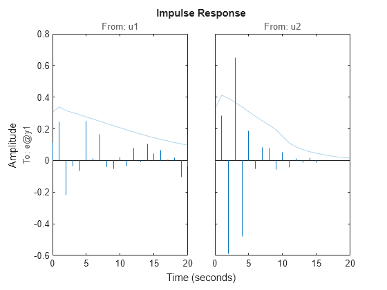
residplots a bode plot of the frequency response from the input signals to the residuals. The 99% confidence region marking statistically insignificant response is shown as a region around the x-axis.
To change display options, right-click the plot to access the context menu. For more details about the menu, see Tips.
resid( computes
and plots the residual of multiple identified models Data,sys1,...,sysn)sys1,...,sysn.
Examples
Input Arguments
Output Arguments
Tips
Right-clicking the plot opens the context menu, where you can access the following options:
Systems — Select systems to view the residual correlation or response plots. By default, all systems are plotted.
Show Confidence Region — View the 99% confidence region marking statistically insignificant correlations. Applicable only for the correlation plots.
Data Experiment — For multi-experiment data only. Toggle between data from different experiments.
Characteristics — View data characteristics. Not applicable for correlation plots.
Peak Response — View peak response of the data.
Confidence Region — View the 99% confidence region marking statistically insignificant response.
Show — Applicable only for frequency-response plots.
Magnitude — View magnitude of frequency response.
Phase — View phase of frequency response.
I/O Grouping — For datasets containing more than one input or output channel. Select grouping of input and output channels on the plot. Not applicable for correlation plots.
None — Plot input-output channels in their own separate axes.
All — Group all input channels together and all output channels together.
I/O Selector — For datasets containing more than one input or output channel. Select a subset of the input and output channels to plot. By default, all output channels are plotted.
Grid — Add grids to the plot.
Normalize — Normalize the y-scale of all data in the plot. Not applicable for frequency-response data.
Full View — Return to full view. By default, the plot is scaled to full view.
Initial Condition — Specify handling of initial conditions.
Specify as one of the following:
Estimate — Treat the initial conditions as estimation parameters.
Zero — Set all initial conditions to zero.
Absorb delays and estimate — Absorb nonzero delays into the model coefficients and treat the initial conditions as estimation parameters. Use this option for discrete-time models only.
Properties — Open the Property Editor dialog box to customize plot attributes.
References
[1] Ljung, L. System Identification: Theory for the User. Upper Saddle River, NJ: Prentice-Hall PTR, 1999, Section 16.6.
Version History
Introduced before R2006a


