comparisonPlot

Class: matlab.perftest.TimeResult
Package: matlab.perftest

Create plot to compare baseline and measurement test results

Since R2019b

Syntax

comparisonPlot(Baseline,Measurement)

comparisonPlot(Baseline,Measurement,stat)

comparisonPlot(___,Name,Value)

cp = comparisonPlot(___)

Description

comparisonPlot(Baseline,Measurement) creates a plot that visually compares each TimeResult object in the arrays Baseline and Measurement. The comparison is based on the minimum of sample measurement times.

comparisonPlot(Baseline,Measurement,stat) specifies the statistic applied to the sample measurement times of each TimeResult object in Baseline and Measurement.

comparisonPlot(___,Name,Value) creates a comparison plot with additional options specified by one or more Name,Value pair arguments. For example, comparisonPlot(Baseline,Measurement,'Scale','linear') creates a plot with a linear scale for the x- and y-axes.

cp = comparisonPlot(___) returns the ComparisonPlot object, specified as an instance of the matlab.unittest.measurement.chart.ComparisonPlot class. Use cp to modify the properties of a specific comparison plot after you create it.

Input Arguments

Baseline — Results from running primary time experiment

matlab.perftest.TimeResult array

Results from running a primary time experiment on a test suite, specified as a TimeResult array. Baseline must have the same length as Measurement.

Measurement — Results from running secondary time experiment

matlab.perftest.TimeResult array

Results from running a secondary time experiment on a test suite, specified as a TimeResult array. Measurement must have the same length as Baseline.

stat — Statistic applied to sample measurement times

'min' (default) | 'max' | 'mean' | 'median'

Statistic applied to the sample measurement times of each TimeResult object in Baseline and Measurement, specified as 'min', 'max', 'mean', or 'median'.

Name-Value Arguments

Specify optional pairs of arguments as Name1=Value1,...,NameN=ValueN, where Name is the argument name and Value is the corresponding value. Name-value arguments must appear after other arguments, but the order of the pairs does not matter.

Before R2021a, use commas to separate each name and value, and enclose Name in quotes.

Example: cp = comparisonPlot(Baseline,Measurement,'SimilarityTolerance',0.05,'Scale','linear')

Scale — Scale of x- and y-axes

'log' (default) | 'linear'

Scale of the x- and y-axes of the ComparisonPlot object, specified as 'log' or 'linear'.

SimilarityTolerance — Allowable deviation of statistics ratio from one

0.1 (default) | numeric scalar

Allowable deviation of the statistics ratio from one, for a pair of similar performance tests, specified as a numeric value between 0 and 1.

SimilarityTolerance specifies the borders of a shaded region in the comparison plot. Data points that fall inside this region represent similar Baseline and Measurement entries.

Parent — Parent container

Figure object (default) | Panel object | Tab object

Parent container in which to plot, specified as a Figure object created with either the figure or uifigure function, a Panel object created with the uipanel function, or a Tab object created with the uitab function.

Examples

Visually Compare Sorting Algorithm Performance

Visualize the computational complexity of two sorting algorithms, bubble sort and merge sort, which sort list elements in ascending order. Bubble sort is a simple sorting algorithm that repeatedly steps through a list, compares adjacent pairs of elements, and swaps elements if they are in the wrong order. Merge sort is a "divide and conquer" algorithm that takes advantage of the ease of merging sorted sublists into a new sorted list.

In your current folder, save the following code in bubbleSort.m.

function y = bubbleSort(x)
% Sorting algorithm with O(n^2) complexity
n = length(x);
swapped = true;

while swapped
    swapped = false;
    for i = 2:n
        if x(i-1) > x(i)
            temp = x(i-1);
            x(i-1) = x(i);
            x(i) = temp;
            swapped = true;
        end
    end
end

y=x;
end

Save the following code in mergeSort.m.

function y = mergeSort(x)
% Sorting algorithm with O(n*logn) complexity
y = x; % A list of one element is considered sorted

if length(x) > 1
    mid = floor(length(x)/2);
    L = x(1:mid);
    R = x((mid+1):end);
    
    % Sort left and right sublists recursively
    L = mergeSort(L);
    R = mergeSort(R);
    
    % Merge the sorted left (L) and right (R) sublists
    i = 1;
    j = 1;
    k = 1;
    while i <= length(L) && j <= length(R)
        if L(i) < R(j)
            y(k) = L(i);
            i = i + 1;
        else
            y(k) = R(j);
            j = j + 1;
        end
        k = k + 1;
    end
    
    % At this point, either L or R is empty
    while i <= length(L)
        y(k) = L(i);
        i = i + 1;
        k = k + 1;
    end
    
    while j <= length(R)
        y(k) = R(j);
        j = j + 1;
        k = k + 1;
    end
end

end

Create the following parameterized test class, TestSort, which compares the performance of the bubble sort and merge sort algorithms. The len property contains the number of list elements you want to test.

classdef TestSort < matlab.perftest.TestCase
    properties
        Data
        SortedData
    end
    
    properties(ClassSetupParameter)
        % Create 25 logarithmically spaced values between 10^2 and 10^4
        len = num2cell(round(logspace(2,4,25)));
    end
    
    methods(TestClassSetup)
        function ClassSetup(testCase,len)
            orig = rng;
            testCase.addTeardown(@rng,orig)
            rng('default')
            testCase.Data = rand(1,len);
            testCase.SortedData = sort(testCase.Data);
        end
    end
    
    methods(Test)
        function testBubbleSort(testCase)
            while testCase.keepMeasuring
                y = bubbleSort(testCase.Data);
            end
            testCase.verifyEqual(y,testCase.SortedData);
        end
        
        function testMergeSort(testCase)
            while testCase.keepMeasuring
                y = mergeSort(testCase.Data);
            end
            testCase.verifyEqual(y,testCase.SortedData);
        end
        
    end
end

Run performance tests for all test elements that correspond to the 'testBubbleSort' method, and save the results in the Baseline array. Your results might vary from the results shown.

Baseline = runperf('TestSort','ProcedureName','testBubbleSort');

Running TestSort
.......... .......... .......... .......... ..........
.......... .......... .......... .......... ..........
.......... .......... .......... .......... ..........
.......... .......... .......... .......... ..........
.......... .......... .......... .......... ..........
.......... .......... .....
Done TestSort
__________

Run performance tests for all elements that correspond to the 'testMergeSort' method, and save the results in the Measurement array.

Measurement = runperf('TestSort','ProcedureName','testMergeSort');

Running TestSort
.......... .......... .......... .......... ..........
.......... .......... .......... .......... ..........
.......... .......... .......... .......... ..........
.......... .......... .......... .......... ..........
Done TestSort
__________

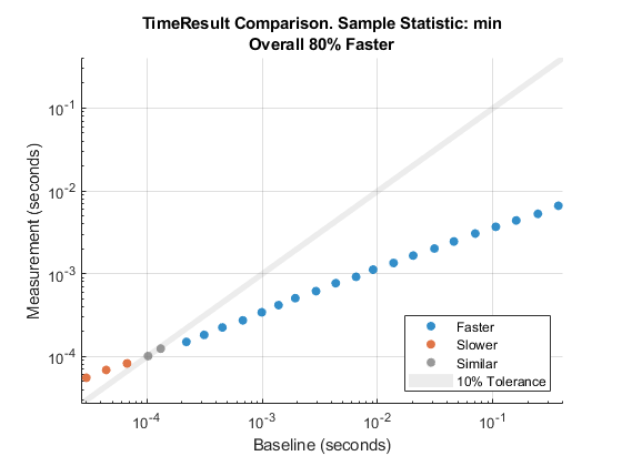
Visually compare the minimum of the MeasuredTime column in the Samples table for each corresponding pair of Baseline and Measurement objects.

comparisonPlot(Baseline,Measurement);

In this comparison plot, most data points are blue because they are below the shaded similarity region. This result indicates the superior performance of merge sort for the majority of test cases. However, for small enough lists, bubble sort performs better than or comparable to merge sort, as shown by the orange and gray points on the plot.

As a comparison summary, the plot reports a 78% performance improvement due to merge sort. This value is the geometric mean of the improvement percentages corresponding to all data points. If the comparison plot contained invalid data points, a comparison summary would not be generated.

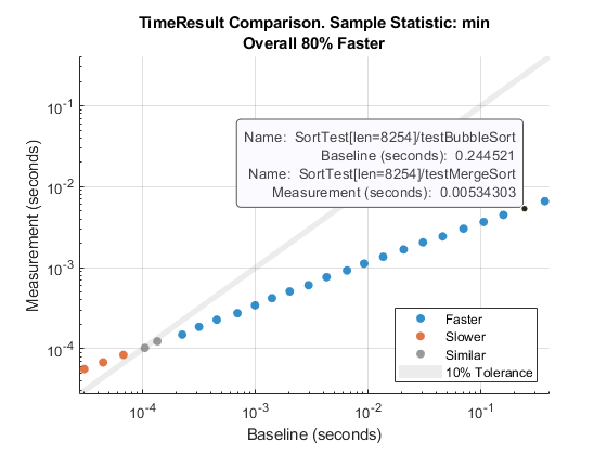
You can press or hover over any data point to view detailed information about the time measurement results being compared.

To study the worst-case sorting algorithm performance for different list lengths, create a comparison plot based on the maximum of sample measurement times.

comparisonPlot(Baseline,Measurement,'max');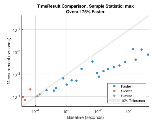

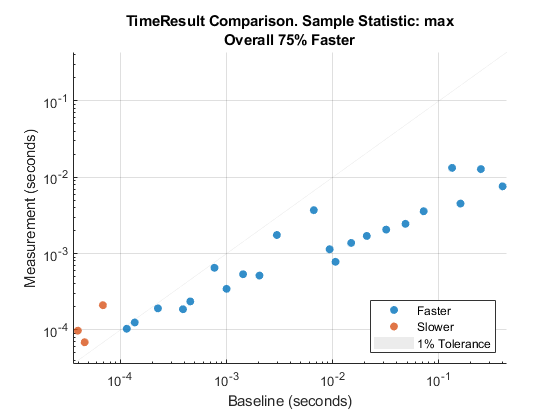
Reduce SimilarityTolerance to 0.01 when comparing the maximum of sample measurement times. Return the ComparisonPlot object in cp so that you can modify its properties later.

cp = comparisonPlot(Baseline,Measurement,'max','SimilarityTolerance',0.01);

Version History

Introduced in R2019b