Export Verilog-A module from Rational Function
This example shows how to use RF Toolbox™ functions to generate a Verilog-A module that models the high-level behavior of a high-speed backplane. First, it reads the single-ended 4-port S-parameters for a differential high-speed backplane and converts them to 2-port differential S-parameters. Then, it computes the transfer function of the differential circuit and fits a rational function to the transfer function. Next, the example exports a Verilog-A module that describes the model. Finally, it plots the unit step response of the generated Verilog-A module in a third-party circuit simulation tool.
Use Rational Function Object to Describe High-Level Behavior of High-Speed Backplane
Read a Touchstone® data file, default.s4p, into an sparameters object. The parameters in this data file are the 50-ohm S-parameters of a single-ended 4-port passive circuit, measured at 1496 frequencies ranging from 50 MHz to 15 GHz. Then, extract the single-ended 4-port S-parameters from the data stored in the Parameters property of the sparameters object, use the s2sdd function to convert them to differential 2-port S-parameters, and use the s2tf function to compute the transfer function of the differential circuit. Then, use the rationalfit function to generate an rfmodel.rational object that describes the high-level behavior of this high-speed backplane. The rfmodel.rational object is a rational function object that expresses the circuit's transfer function in closed form using poles, residues, and other parameters, as described in the rationalfit reference page.
filename = 'default.s4p';
backplane = sparameters(filename);
data = backplane.Parameters;
freq = backplane.Frequencies;
z0 = backplane.Impedance;
Convert to 2-port differential S-parameters.
diffdata = s2sdd(data);
diffz0 = 2*z0;
difftf = s2tf(diffdata,diffz0,diffz0,diffz0);
Fit the differential transfer function into a rational function.
fittol = -30;           % Rational fitting tolerance in dB
delayfactor = 0.9;      % Delay factor
rationalfunc = rationalfit(freq,difftf,fittol,'DelayFactor',delayfactor)
rationalfunc =
   rfmodel.rational with properties:

        A: [20×1 double]
        C: [20×1 double]
        D: 0
    Delay: 6.0172e-09
     Name: 'Rational Function'
Export Rational Function Object as Verilog-A Module
Use the writeva method of the rfmodel.rational object to export the rational function object as a Verilog-A module, called samplepassive1, that describes the rational model. The input and output nets of samplepassive1 are called line_in and line_out. The predefined Verilog-A discipline, electrical, describes the attributes of these nets. The format of numeric values, such as the Laplace transform numerator and denominator coefficients, is %12.10e. The electrical discipline is defined in the file disciplines.vams, which is included in the beginning of the samplepassive1.va file.
workingdir = tempname;
mkdir(workingdir)
writeva(rationalfunc, fullfile(workingdir,'samplepassive1'), ...
    'line_in', 'line_out', 'electrical', '%12.10e', 'disciplines.vams');
type(fullfile(workingdir,'samplepassive1.va'));// Module: samplepassive1
// Generated by MATLAB(R) 26.1 and the RF Toolbox 26.1.
// Generated on: 19-Apr-2026 12:21:33
`include "disciplines.vams"
module samplepassive1(line_in, line_out);
electrical line_in, line_out;
electrical node1;
real nn1[0:1], nn2[0:1], nn3[0:1], nn4[0:1], nn5[0:1], nn6[0:1], nn7[0:1], nn8[0:1], nn9[0:1], nn10[0:0], nn11[0:0];
real dd1[0:2], dd2[0:2], dd3[0:2], dd4[0:2], dd5[0:2], dd6[0:2], dd7[0:2], dd8[0:2], dd9[0:2], dd10[0:1], dd11[0:1];
analog begin
@(initial_step) begin
nn1[0] = -3.8392614832e+18;
nn1[1] = 5.2046393014e+07;
dd1[0] = 2.8312609831e+21;
dd1[1] = 3.5124823781e+09;
dd1[2] = 1.0000000000e+00;
nn2[0] = -2.0838483814e+19;
nn2[1] = 5.3487174018e+08;
dd2[0] = 1.8020362314e+21;
dd2[1] = 7.8266367089e+09;
dd2[2] = 1.0000000000e+00;
nn3[0] = 1.7726270794e+19;
nn3[1] = 2.5185716022e+09;
dd3[0] = 1.2157471895e+21;
dd3[1] = 8.1132784895e+09;
dd3[2] = 1.0000000000e+00;
nn4[0] = 2.3112282793e+20;
nn4[1] = 9.2690544437e+08;
dd4[0] = 7.9582429152e+20;
dd4[1] = 1.1379108659e+10;
dd4[2] = 1.0000000000e+00;
nn5[0] = 8.9321469721e+19;
nn5[1] = -1.4945928109e+10;
dd5[0] = 4.1473706594e+20;
dd5[1] = 1.1346735824e+10;
dd5[2] = 1.0000000000e+00;
nn6[0] = -3.5180951909e+20;
nn6[1] = -1.9895507212e+10;
dd6[0] = 1.9080843811e+20;
dd6[1] = 1.0434555792e+10;
dd6[2] = 1.0000000000e+00;
nn7[0] = -1.0593240107e+20;
nn7[1] = 1.9248932577e+10;
dd7[0] = 6.1152960549e+19;
dd7[1] = 1.0001203231e+10;
dd7[2] = 1.0000000000e+00;
nn8[0] = 5.4441539402e+16;
nn8[1] = -9.7818749687e+06;
dd8[0] = 4.3821946493e+19;
dd8[1] = 6.6700188623e+08;
dd8[2] = 1.0000000000e+00;
nn9[0] = 2.2556903052e+16;
nn9[1] = 7.9711163023e+06;
dd9[0] = 2.1228807651e+19;
dd9[1] = 4.9531801417e+08;
dd9[2] = 1.0000000000e+00;
nn10[0] = 1.1592988960e+10;
dd10[0] = 3.0829914556e+09;
dd10[1] = 1.0000000000e+00;
nn11[0] = 1.2852839051e+08;
dd11[0] = 5.9779845807e+08;
dd11[1] = 1.0000000000e+00;
end
V(node1) <+ laplace_nd(V(line_in), nn1, dd1);
V(node1) <+ laplace_nd(V(line_in), nn2, dd2);
V(node1) <+ laplace_nd(V(line_in), nn3, dd3);
V(node1) <+ laplace_nd(V(line_in), nn4, dd4);
V(node1) <+ laplace_nd(V(line_in), nn5, dd5);
V(node1) <+ laplace_nd(V(line_in), nn6, dd6);
V(node1) <+ laplace_nd(V(line_in), nn7, dd7);
V(node1) <+ laplace_nd(V(line_in), nn8, dd8);
V(node1) <+ laplace_nd(V(line_in), nn9, dd9);
V(node1) <+ laplace_nd(V(line_in), nn10, dd10);
V(node1) <+ laplace_nd(V(line_in), nn11, dd11);
V(line_out) <+ absdelay(V(node1), 6.0171901584e-09);
end
endmodule
Plot Unit Step Response of Generated Verilog-A Module
Many third-party circuit simulation tools support the Verilog-A standard. These tools simulate standalone components defined by Verilog-A modules and circuits that contain these components. The following figure shows the unit step response of the samplepassive1 module. The figure was generated with a third-party circuit simulation tool.
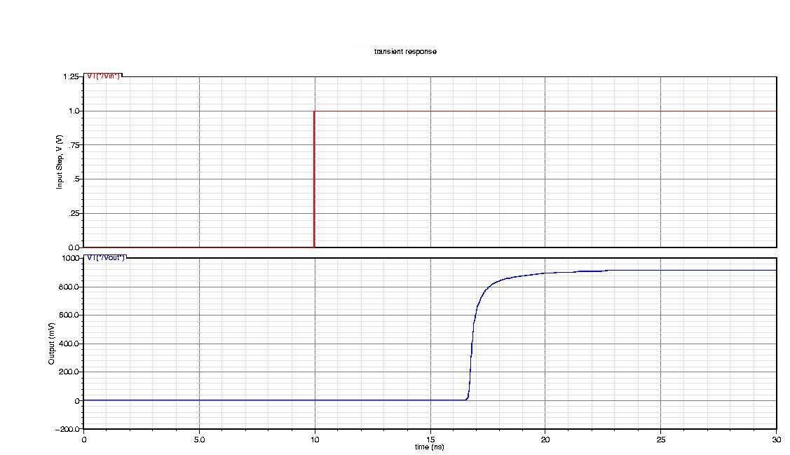
Figure 1: The unit step response.
delete(fullfile(workingdir,'samplepassive1.va'));
rmdir(workingdir)