Feature Selection Based on Deep Learning Interpretability for Signal Classification Applications
This example demonstrates how to use the locally interpretable model-agnostic explanations (LIME) technique to interpret the decision-making process of a deep learning network. The example uses the insight obtained from the network's decision rationale to perform feature selection to reduce the size of the data and the network complexity while maintaining similar levels of accuracy.
In this example, you create and train a neural network to classify four classes of simulated signal data:
Sine waves of a single frequency
Superpositions of three sine waves
Signals with broad Gaussian peaks
Signals with Gaussian pulses
To make this problem more realistic, the example adds a low-frequency background tone and high-frequency noise as impairments to the signals.
Generate Waveforms and Features
Generate 200 realizations for each one of the four signal classes. Each signal has 501 samples. This example uses the helper function generateData to generate the noisy time series. The helper functions used in this example are attached as supporting files.
numObsPerClass = 200;
[signals,labels] = generateData(numObsPerClass);
Plot Generated Data
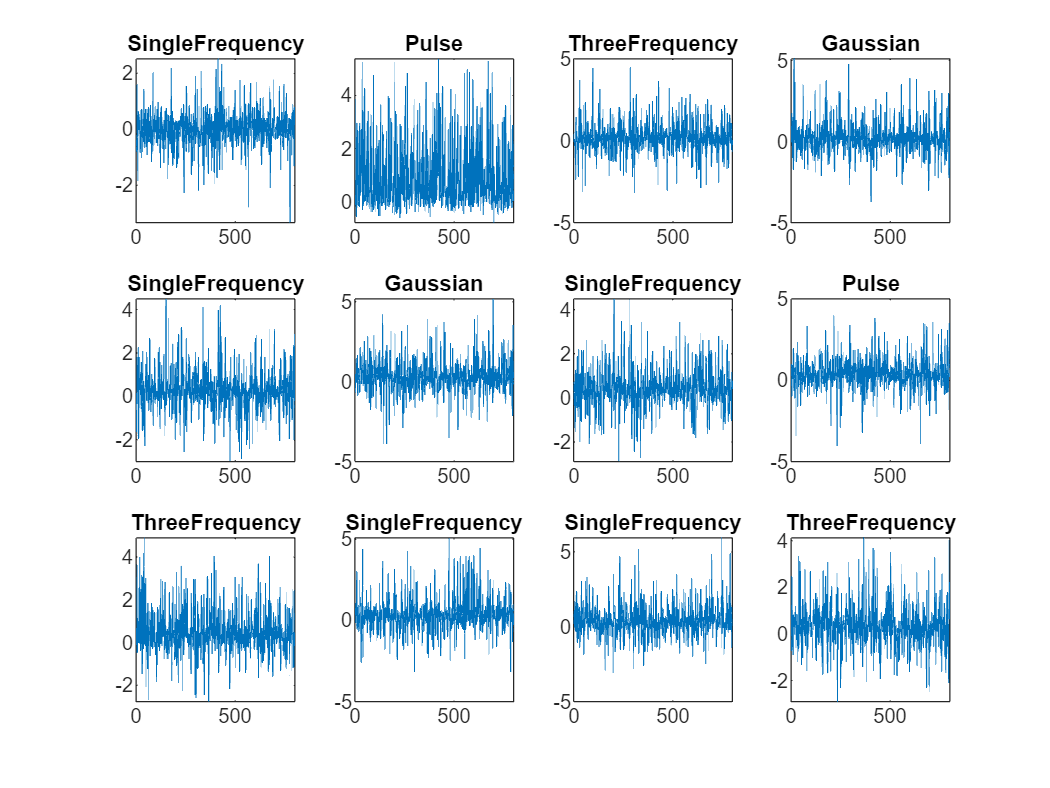
Plot a subset of the generated signals. Distinguishing any differentiating features in the time domain signals is challenging because the noise is comparable in magnitude to the signal content. A common approach to solve this problem is to extract features from the signals to enhance their particular characteristics. Figuring out what are the best features that best describe the signals is a difficult problem. A typical approach is to obtain as many features as possible and try out all the features at once or in different combinations. The next sections show how to easily extract features from the signals using feature extraction objects and how to use a deep network and interpretability techniques to select only the most significant features to reduce the network complexity.
numPlots = 12;
tiledlayout(3,4)
for ii = 1:numPlots
    nexttile
    plot(signals(ii,:))
    title(labels(ii))
end
Extract Features
Use signal feature extractors to extract features from the signals. Framing the signal into smaller segments enables more efficient computations and improves temporal resolution. As an initial blind selection, choose a variety of different time, frequency, and time-frequency features. Combine them together to form a feature tensor.
timeFE = signalTimeFeatureExtractor(SampleRate=100, ...
    FrameSize=100, ...
    FrameOverlapLength=30, ...
    RMS=false, ...
    CrestFactor=true, ...
    ImpulseFactor=true, ...
    StandardDeviation=true, ...
    SNR=true, ...
    ShapeFactor=true);
[timeFeature,infoT] = extract(timeFE,signals);
freqFE = signalFrequencyFeatureExtractor(SampleRate=100, ...
    FrameSize=100, ...
    FrameOverlapLength=30, ...
    MeanFrequency=true, ...
    BandPower=true, ...
    PeakLocation=true, ...
    PeakAmplitude=true, ...
    PowerBandwidth=true);
[freqFeature,infoF] = extract(freqFE,signals);
timeFreqFE = signalTimeFrequencyFeatureExtractor(SampleRate=100, ...
    FrameSize=100, ...
    FrameOverlapLength=30, ...
    SpectralKurtosis=true, ...
    SpectralFlatness=true, ...
    InstantaneousFrequency=true, ...
    InstantaneousEnergy=false, ...
    InstantaneousBandwidth=true, ...
    TimeSpectrum=true, ...
    TFRidges=true, ...
    WaveletEntropy=true, ...
    MeanEnvelopeEnergy=false);
[TimeFreqFeature,infoTF] = extract(timeFreqFE,signals);
features = [timeFeature,freqFeature,TimeFreqFeature];
The final feature tensor is 6-by-170-by-800. These dimensions represent the number of frames, features, and signal, respectively.
whos featuresName Size Bytes Class Attributes features 6x170x800 6528000 double
View which of the 170 channels corresponds to which feature's specific channel.
numChannel = size(features,2);
featureInfoTable = helperGetFeatureInfoTable({infoT,infoF,infoTF},numChannel);
featureInfoTable(1:10,:)ans=10×1 table
Feature
____________________
"StandardDeviation1"
"ShapeFactor1"
"SNR1"
"CrestFactor1"
"ImpulseFactor1"
"MeanFrequency1"
"BandPower1"
"PowerBandwidth1"
"PeakAmplitude1"
"PeakLocation1"
Prepare Data for Training
Use the splitlabels function to divide the data into training, validation and test data. Use 70% of the data for training, 10% for validation, and 20% for testing.
splitIndices = splitlabels(labels,[0.7,0.1,0.2]);

featureTrain = features(:,:,splitIndices{1});
labelsTrain = labels(splitIndices{1});

featureVal = features(:,:,splitIndices{2});
labelsVal = labels(splitIndices{2});

featureTest = features(:,:,splitIndices{3});
labelsTest = labels(splitIndices{3});
Normalize Features
Due to the significant differences in the numerical ranges and distributions of various features, normalization is often beneficial in enabling the network to work effectively with all different kinds of features.
Here, it is important to apply normalization to each feature separately for scale consistency, while considering the full dataset for each feature to ensure the proper distribution assessment. Use the batchnorm function, which normalizes a mini-batch of data across all observations for each channel independently.
To avoid using prior knowledge of statistics from the validation and test data, use only training data to calculate normalization statistics. Use the estimated statistics to normalize the other data.
numChannel = size(features,2);
offset = zeros(numChannel,1);
scaleFactor = ones(numChannel,1);
[featureTrainNorm,estMu,estSigmaSq] = batchnorm(dlarray(featureTrain), ...
    offset,scaleFactor, ...
    DataFormat="TCB");
featureValNorm = batchnorm(dlarray(featureVal), ...
    offset,scaleFactor, ...
    estMu,estSigmaSq, ...
    DataFormat="TCB");
featureTestNorm = batchnorm(dlarray(featureTest), ...
    offset,scaleFactor, ...
    estMu,estSigmaSq, ...
    DataFormat="TCB");
featureTrainNorm = extractdata(featureTrainNorm);
featureValNorm = extractdata(featureValNorm);
featureTestNorm = extractdata(featureTestNorm);
Visualize Normalized Features
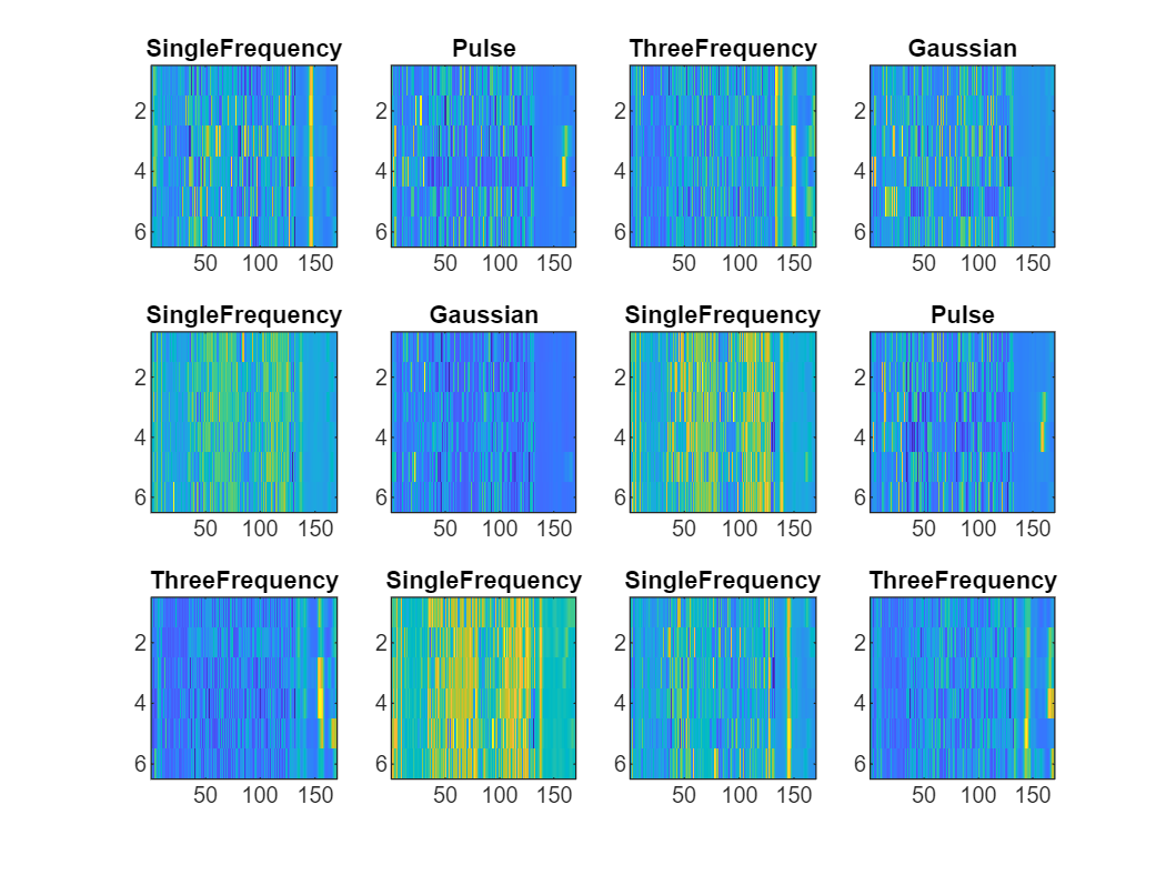
Plot the features of the noisy data.
Features from different types of signals appear distinct. However, it is still challenging to determine which features are most relevant for classification. In the next section, use the features as images to train a simple convolutional neural network classifier.
figure
clims = [0 8];
tiledlayout(3,4)
for ii = 1:12
    nexttile
    imagesc(featureTrainNorm(:,:,ii))
    title(labels(ii))
end
Train a Classification Network
Create a simple convolutional neural network with a single convolutional layer. Note that we have a 5-by-1 convolutional kernel. Thus you can convolve only along the first (time-frame) dimension. Avoid convolving along the feature dimension because the features do not have a clear spatial relationship. In other words, adjacent features are not necessarily correlated.
dropoutProb = 0.2;
numFilters = 8;
numClasses = length(unique(labels));
inputSize = size(featureTrainNorm,[1 2])
inputSize = 1×2

     6   170
layers = [ ...
    imageInputLayer(inputSize)
    convolution2dLayer([5,1],numFilters,Padding="same")
    batchNormalizationLayer
    reluLayer
    dropoutLayer(dropoutProb)
    fullyConnectedLayer(numClasses)
    softmaxLayer];
Define options for training using the ADAM optimizer.
options = trainingOptions("adam", ...
    Shuffle="every-epoch", ...
    Plots="training-progress", ...
    Metrics="accuracy", ...
    Verbose=false, ...
    MiniBatchSize=50, ...
    MaxEpochs=100, ...
    validationData={featureValNorm,labelsVal}, ...
    InputDataFormats="SSBC", ...
    ExecutionEnvironment="cpu");
Train Network
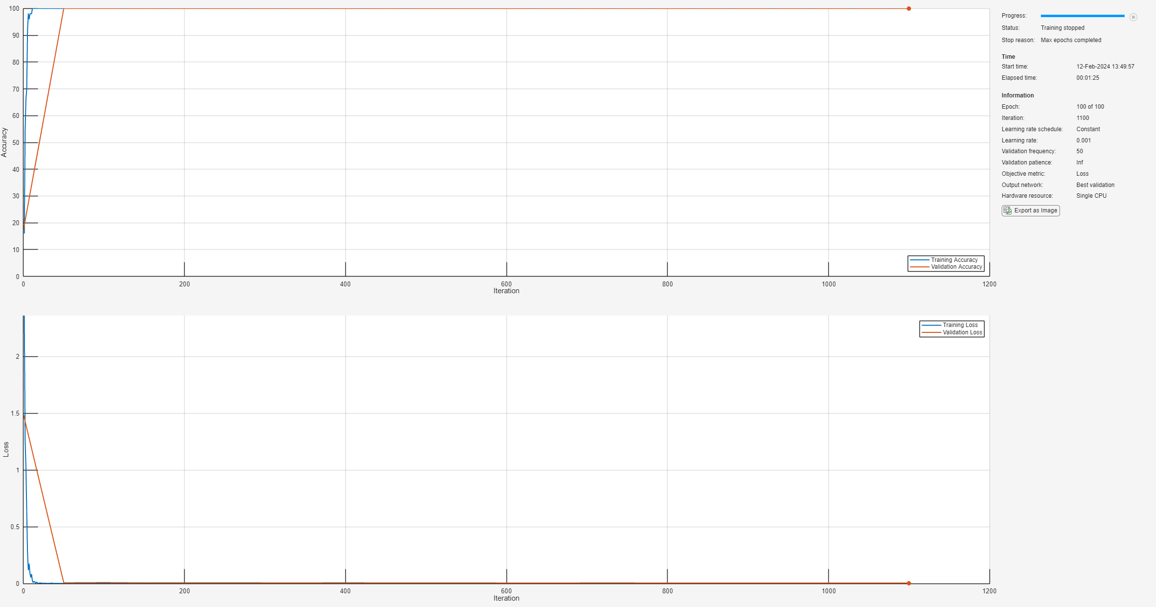
Train the network to classify the signals.
net = trainnet(featureTrainNorm, ...
    labelsTrain, ...
    layers, ...
    "crossentropy", ...
    options);
Test Performance
Classify the testing observations using the trained network.
classNames = categories(labelsTrain);
scores= minibatchpredict(net,featureTestNorm,InputDataFormats="SSBC");
labelsPred = scores2label(scores,classNames);
Investigate the network performance by plotting a confusion matrix with confusionchart.
figure
confusionchart(labelsTest,labelsPred,Normalization="row-normalized")
The network accurately classifies the validation data, with close to 100% accuracy for most of the classes.
Use LIME to Investigate Classification Results
Use the imageLIME function on validation data to identify the features that the model prioritizes when making classification decisions.
LIME is a technique used to explain what features are most important for classification. The LIME technique segments an image into several features and generates synthetic observations by randomly including or excluding features. Each pixel in an excluded feature is replaced with the value of the average image pixel. The network classifies these synthetic observations and uses the resulting scores for the predicted class, along with the presence or absence of a feature, as responses and predictors to train a regression problem with a simpler model. In this example, the model is a regression tree. The regression tree tries to approximate the behavior of the network on a single observation. It learns which features are important and significantly impact the class score.
Define Custom Segmentation Map
By default, imageLIME uses superpixel segmentation to divide the image into features. This option works well for photographic images, but is less effective for other types of images, such as spectrograms or feature matrix data. You can specify a custom segmentation map by setting the "Segmentation" name-value argument to a numeric matrix the same size as the input data, where each element is an integer corresponding to the index of the feature associated with each point of the input.
To emphasize the x-dimension (feature channel) over the y-dimension (time frame) in the feature matrix data, create a segmentation map with size 1x170. This map assigns each feature channel to an individual segment. Next, upscale this map to match the image size by applying the imresize function and selecting "nearest" as the upsampling method.
inputSize = size(features,[1,2]);
segmentationMap = 1:170;
segmentationMap = imresize(segmentationMap,inputSize,"nearest");
Compute LIME Map
scoreMapAll = zeros(size(featureValNorm));
for ii = 1:length(labelsVal)
    channel =  find(classNames==labelsVal(ii));
    scoreMap = imageLIME(net,featureValNorm(:,:,ii),channel, ...
        Segmentation=segmentationMap, ...
        NumSamples=4000);
    scoreMapAll(:,:,ii) = rescale(scoreMap);
end
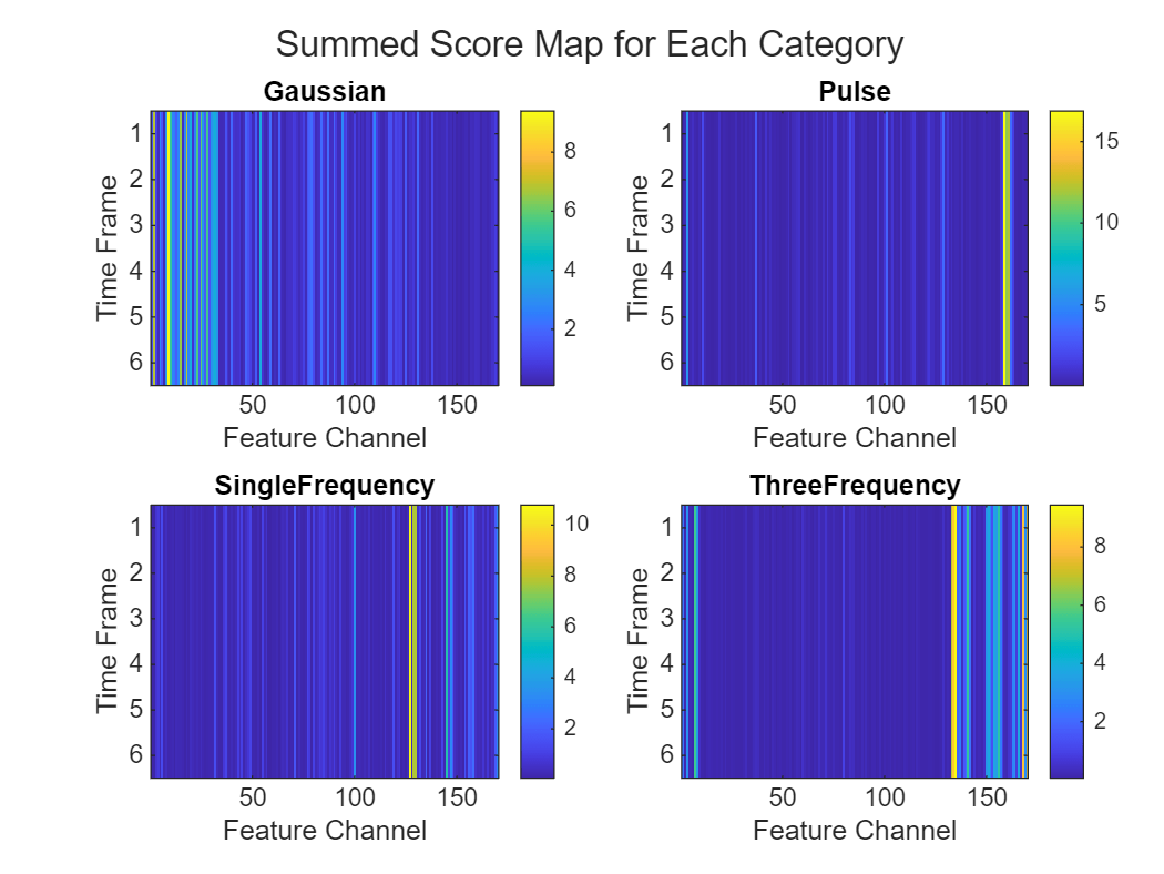
The score map below shows time frames on the y-axis and feature channels on the x-axis. Higher scores indicate features that are more important for the classification.
obsToShowPerClass = 2;
fig = figure;
tiledlayout(length(classNames),obsToShowPerClass*2,TileSpacing="compact");
for ii = 1:length(classNames)
    idx = find(labelsVal==classNames(ii),obsToShowPerClass);
    for jj = 1:obsToShowPerClass
        % Feature Matrix subplot
        nexttile
        imagesc(featureValNorm(:,:,idx(jj)));
        if jj==1
            ylabel(string(classNames(ii)));
        end
        title("Feature Matrix")
        % Score Map subplot
        nexttile
        imagesc(scoreMapAll(:,:,idx(jj)));
        title("Score Map")
    end
end
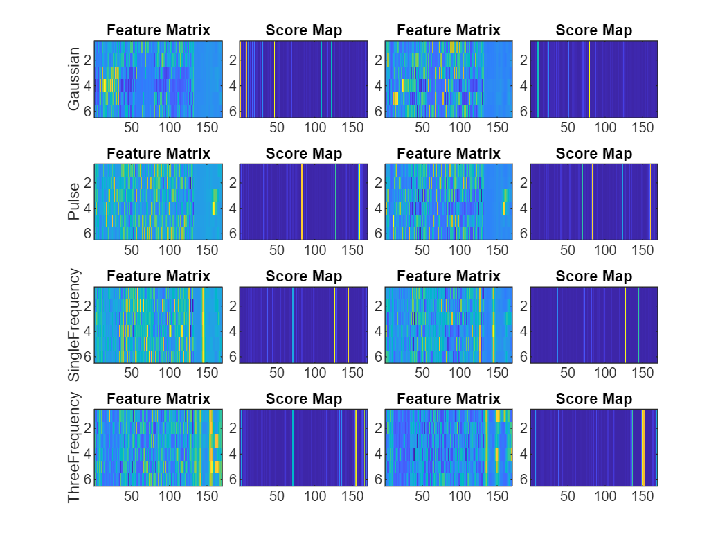
Sum the importance maps across all validation observations to obtain an overall importance map for each class. Now it is clear that the network decision-making process concentrates on a few key features overall for a specific category.
summedScoreMaps = struct();
for ii = 1:length(classNames)
    idx = find(labelsVal==classNames{ii});
    summedScoreMaps.(classNames{ii}) = sum(scoreMapAll(:,:,idx),3);
end
t = tiledlayout(2,2,TileSpacing="compact");
for ii = 1:length(classNames)
    scoreMapSum = summedScoreMaps.(classNames{ii});
    nexttile
    imagesc(scoreMapSum);
    colorbar
    title(classNames{ii})
    xlabel("Feature Channel")
    ylabel("Time Frame")
end
title(t,"Summed Score Map for Each Category");
Find the Most Important Features
Select the most important feature channel for each category based on LIME importance score map. Sum the scores over each time frame to get a single score per feature channel and select the feature with the highest score as most important.
numTop = 1;
topIdxList = zeros(length(classNames), 1);
t = tiledlayout(2,2,TileSpacing="compact",Padding="compact");
for ii = 1:length(classNames)
    category = fieldnames(summedScoreMaps);
    scoreMapSum = summedScoreMaps.(category{ii});
    % Calculate score per feature
    scorePerFeature = sum(scoreMapSum, 1);
    % Get top features
    [~, topIdx] = maxk(scorePerFeature, numTop);
    topIdxList(ii) = topIdx(1);
    % Plotting
    nexttile;
    bar(scorePerFeature);
    hold on;
    stem(topIdx, scorePerFeature(topIdx),"diamond","filled");
    if topIdx<85
        aligment = "left";
    else
        aligment = "right";
    end
    text(topIdx,scorePerFeature(topIdx), ...
        "   "+featureInfoTable{topIdx,1}+"   ", ...
        HorizontalAlignment=aligment)
    hold off
    xlabel("Feature Channel Index");
    ylabel("Importance Score");
    title(classNames{ii});
    ylim([0 max(scorePerFeature+10)])
    grid on
    box on
end
title(t,"Importance Score for Each Category");

Retrain the Network with Only Selected Features
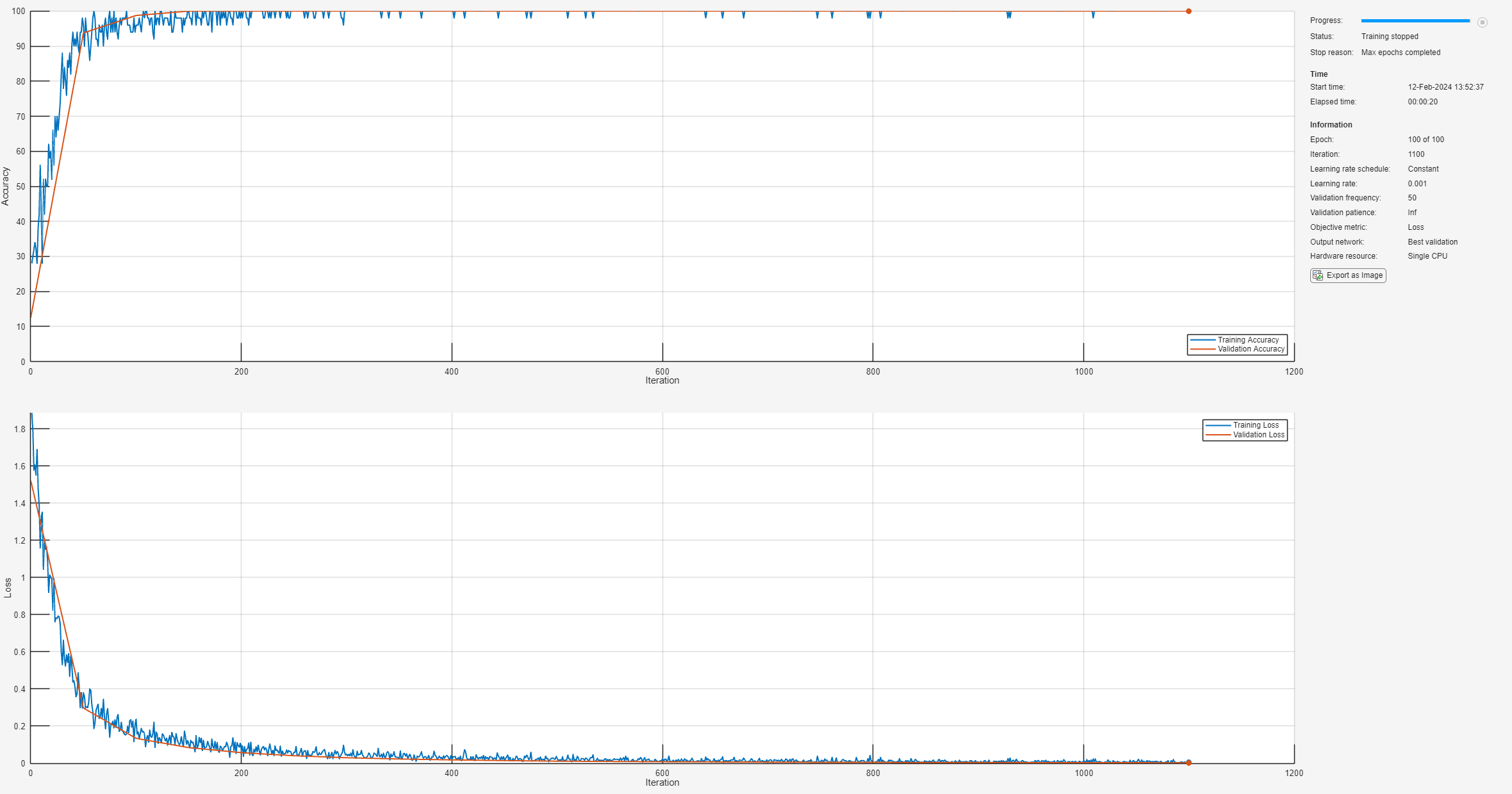
Retrain the network using only the most important selected features. The input size decreases from 6-by-170 to only 6-by-4 – an over 97% decrease in dimensionality. Furthermore, the time required to classify future data is also significantly reduced.
inputSize = [size(featureTrainNorm,1),length(topIdxList)]
inputSize = 1×2

     6     4
For a relatively fair comparison, maintain the same network and training options. Change only the number of features.
layers2 = [ ...
    imageInputLayer(inputSize)
    convolution2dLayer([5,1],numFilters,Padding="same")
    batchNormalizationLayer
    reluLayer
    dropoutLayer(dropoutProb)
    fullyConnectedLayer(numClasses)
    softmaxLayer];
options = trainingOptions("adam", ...
    Shuffle="every-epoch", ...
    Plots="training-progress", ...
    Metrics="accuracy", ...
    Verbose=false, ...
    MiniBatchSize=50, ...
    MaxEpochs=100, ...
    validationData={featureValNorm(:,topIdxList,:),labelsVal}, ...
    InputDataFormats="SSBC", ...
    ExecutionEnvironment="cpu");
net2 = trainnet(featureTrainNorm(:,topIdxList,:), ...
    labelsTrain, ...
    layers2, ...
    "crossentropy", ...
    options);
Test the retrained network on the testing dataset.
scores= minibatchpredict(net2,featureTestNorm(:,topIdxList,:),InputDataFormats="SSBC");
labelsPred = scores2label(scores,classNames);
figure
confusionchart(labelsTest,labelsPred,Normalization="row-normalized")
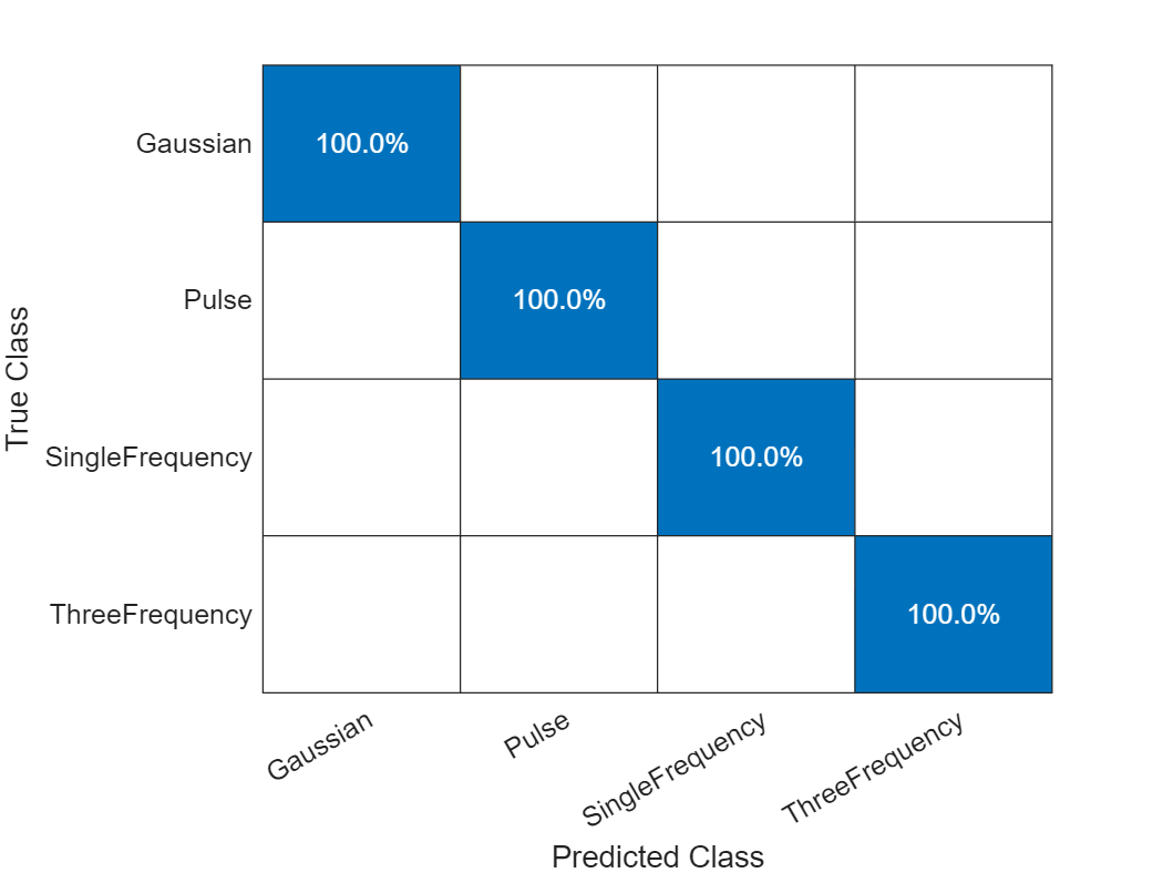
Even though the number of features is less than 5% of the original, the model's performance has not significantly changed.
Compare with Random Feature Selection
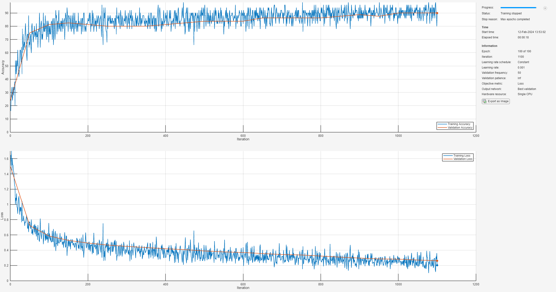
Compare the feature selection approach to show that the best feature selection has superior performance to a random feature selection.
rng("default")
idxRand = randperm(size(features,2),length(topIdxList));
List the randomly selected features.
featureInfoTable(idxRand(:),:)
ans=4×1 table
          Feature
    ____________________

    "TimeSpectrum7"
    "TimeSpectrum22"
    "SpectralKurtosis12"
    "TimeSpectrum21"
Train the network again with random selected features.
options = trainingOptions("adam", ...
    Shuffle="every-epoch", ...
    Plots="training-progress", ...
    Metrics="accuracy", ...
    Verbose=false, ...
    MiniBatchSize=50, ...
    MaxEpochs=100, ...
    validationData={featureValNorm(:,idxRand,:),labelsVal}, ...
    InputDataFormats="SSBC", ...
    ExecutionEnvironment="cpu");
net3 = trainnet(featureTrainNorm(:,idxRand,:), ...
    labelsTrain, ...
    layers2, ...
    "crossentropy", ...
    options);
Test the retrained network on the testing dataset.
scores= minibatchpredict(net3,featureTestNorm(:,idxRand,:),InputDataFormats="SSBC");
labelsPred = scores2label(scores,classNames);
figure
confusionchart(labelsTest,labelsPred,Normalization="row-normalized")
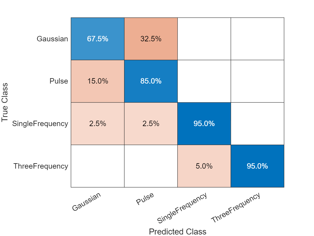
The results are not as good as with the previous, importance-based selection. It's worth mentioning that the randomly selected features do not necessarily always perform worse than those selected through LIME previously. There is a lot of redundant information among the features. The combination selected through LIME is not the only one capable of classifying different types of signals. Through random selection, it's also possible to choose features sufficient for distinguishing signals. However, the effectiveness of this approach is less predictable compared to the systematic methods discussed earlier.
Conclusion
This example demonstrates how to use LIME to examine how a trained classification network makes decisions based on a feature matrix. The example uses importance scores obtained with LIME to select the best features and retrain a network with much less computational complexity and memory requirements but with similar classification performance.
Helper Functions
helperGetFeatureInfoTable – This function collects feature information and forms a table with feature indices and their corresponding feature names.
function featureInfoTable = helperGetFeatureInfoTable(infoArray,nfeatures)
% This function is only intended to support examples in the Signal
% Processing Toolbox. It may be changed or removed in a future release.

featureInfoTable = table(strings(nfeatures, 1),VariableNames="Feature");
% Initialize accumulated indices offset
accIndices = 0;
% Loop through each structure in the infoArray
for i = 1:length(infoArray)
    % Get the current structure
    currInfo = infoArray{i};
    % Loop through each field of the current structure
    fieldNamesList = fieldnames(currInfo);
    for j = 1:numel(fieldNamesList)
        fieldName = fieldNamesList{j};
        currIndices = currInfo.(fieldName);
        indices = currIndices + accIndices;
        % Set the indices rows of the table to the current field name
        % featureInfoTable.Feature(indices) = num2cell(fieldName+string((1:length(indices))'));
        featureInfoTable.Feature(indices) = fieldName+string((1:length(indices))');
    end
    % Update accumulated indices
    accIndices = indices(end);
end
end
See Also
Functions
confusionchart(Deep Learning Toolbox) |minibatchpredict(Deep Learning Toolbox) |scores2label(Deep Learning Toolbox) |trainingOptions(Deep Learning Toolbox) |trainnet(Deep Learning Toolbox)