Optimize LTI System to Meet Frequency-Domain Requirements

This example shows how to use frequency-domain design requirements to optimize the response of an LTI system in the Control System Designer app.

When used with Control System Toolbox™ software, you can place Simulink^® Design Optimization™ design requirements or constraints on plots in the Control System Designer (Control System Toolbox) app. You can include design requirements for response optimization in the frequency-domain and time-domain.

You can specify frequency-domain design requirements to optimize response signals for any model that you design in the Control System Designer app, such as:

Command-line LTI models created with the Control System Toolbox commands
Simulink models that have been linearized using Simulink Control Design™ software

Design Requirements

In this example, you use a linearized version of a Simulink model.

You use optimization methods to design a compensator so that the closed-loop system meets the following design specifications when you excite the system with a unit step input:

Maximum 30-second settling time
Maximum 10% overshoot
Maximum 10-second rise time
Limit of ±0.7 on the actuator signal

Create an LTI Plant Model

In the Simulink model, the plant model is composed of a gain, a limited integrator, a transfer function, and a transport delay block.

Design the compensator for the open-loop transfer function of the linearized model. The linearized plant model is composed of the gain, an unlimited integrator, the transfer function, and a Padé approximation to the transport delay.

To create an open-loop transfer function based on the linearized model, enter the following commands.

w0 = 1;
zeta = 1;
Kint = 0.5;
Tdelay = 1;
[delayNum,delayDen] = pade(Tdelay,1);
integrator = tf(Kint,[1 0]);
transfer_fcn = tf(w0^2,[1 2*w0*zeta w0^2]);
delay_block = tf(delayNum,delayDen);
open_loopTF = integrator*transfer_fcn*delay_block;

If the plant model is an array of models (Control System Toolbox), the controller is designed for a nominal model only. You can also analyze the control design for the remaining models in the array. For more information, see Multimodel Control Design (Control System Toolbox).

Tip

You can directly linearize the Simulink model using Simulink Control Design software.

Open the Control System Designer App

This example uses a root locus diagram to design the response of the open-loop transfer function, open_loopTF. To create a Control System Designer app session with a root locus plot for the open-loop transfer function, use the following command:

controlSystemDesigner('rlocus',open_loopTF)

The Control System Designer app opens, and a Root Locus Editor is displayed. The app lets you design controllers for single-input, single-output (SISO) systems in MATLAB^® and Simulink. For more information, see the Classical Control Design (Control System Toolbox) category.

The app also displays the step response plot of the system. The plot shows the response of the closed-loop system from r (input to the prefilter, F) to y (output of the plant model, G).

To choose the architecture for the control system you are designing, in the app click Edit Architecture. This example uses the default architecture. In this system, the plant model, G, is the open-loop transfer function open_loopTF. The prefilter, F, and the sensor, H, are set to 1, and the compensator, C, is the compensator that is designed using response optimization methods.

Open Optimization Based Tuning Method

There are several possible methods for designing a SISO system; this example uses an automated approach that uses response optimization methods.

To create a response optimization task, in the Tuning Methods drop-down list, select Optimization Based Tuning.

The Response Optimization window has four tabs. Except for the first tab, each tab corresponds to a step in the response optimization process:

Overview — Schematic diagram of the response optimization process.
Compensators — Select and configure the compensator elements that you want to tune. See Select Tunable Compensator Elements.
Design Requirements — Select the design requirements that you want the system to meet after tuning the compensator elements. See Add Design Requirements.
Optimization — Configure optimization options, and view the progress of the response optimization. See Optimize the System Response.

Note

When optimizing responses in the app, you cannot add uncertainty to parameters or compensator elements.

Select Tunable Compensator Elements

You can tune compensator elements or parameters within compensators in your system to meet the design requirements you specify.

To specify the compensator elements to tune:

In the Response Optimization window, select the Compensators tab.
In the Compensators tab, select the check boxes in the Optimize column that correspond to the compensator elements to tune.
In this example, select Gain in the compensator C.

Add Design Requirements

You can use both frequency-domain and time-domain design requirements to tune parameters in a control system.

This example uses the design specifications described in Design Requirements. Create design requirements to meet these specifications:

After you add the design requirements, you can select a subset of requirements for controller design, as described in Select the Design Requirements to Use During Response Optimization. In the Design Requirements tab of the Response Optimization window, you can create design requirements and select the requirements you want to use for optimization.

Settling Time Design Requirement

The first design requirement is to have a settling time of 30 seconds or less. This specification can be represented on a root locus diagram as a constraint on the real parts of the poles of the open-loop system.

To add the settling time design requirement:

In the Design Requirements tab, click Add New Design Requirement. A New Design Requirement dialog box opens.
In this dialog box, you can specify new design requirements, and add them to a new or existing plot.
Add a design requirement to the existing root locus diagram.
1. In the Design requirement type drop-down list, select Settling time.
2. In the Requirement for response drop-down list, select LoopTransfer_C.
3. Specify Settling time as 30 seconds.
4. Click OK.
The settling time design requirement is listed in the Design Requirements tab of the Response Optimization window.
In the app, the design requirement appears on the root locus plot as a vertical line.

Overshoot Design Requirement

The second design requirement is to have a percentage overshoot of 10% or less. This requirement is related to the damping ratio on a root locus diagram. In addition to adding a design requirement with the Add New Design Requirement button, you can also right-click directly on the plots to add the requirement.

To add this design requirement:

In the Control System Designer app, right-click within the white space of the root-locus diagram. Select Design Requirements > New to open the New Design Requirement dialog box.
In the Design requirement type drop-down list, select Percent overshoot.
Specify Percent overshoot as 10.
Click OK.

In the app, the design requirement appears on the root-locus plot as two lines radiating at an angle from the origin.

Rise Time Design Requirement

The third design requirement is to have a rise time of 10 seconds or less. This requirement corresponds to a lower limit on a Bode Magnitude diagram.

To add this design requirement:

In the app, in the Tuning Methods drop-down list, select Bode Editor.
In the Select response to plot dialog box, specify Select Response to Edit as LoopTransfer_C, and click Plot.
A Bode plot is displayed in a Bode Editor.
Right-click within the white space of the open-loop Bode plot, and select Design Requirements > New, to open the New Design Requirement dialog box.
Specify the design requirement to represent the rise time, and add it to the new Bode plot.
1. In the Design requirement type drop-down list, select Lower gain limit.
2. Specify the Frequency range as 1e-2 to 0.17.
3. Specify the Magnitude range as 0 to 0.
4. Click OK.
The design requirement appears on the plot as a horizontal line.

Actuator Limit Design Requirement

The fourth design requirement is to limit the actuator signal to within ±0.7.

To add this design requirement:

In the Response Optimization window, in the Design Requirements, click Add New Design Requirement. A New Design Requirement dialog box opens.
Create a time-domain design requirement to represent the upper limit on the actuator signal, and add it to a new step response plot:
1. In the Design requirement type drop-down list, select Step response upper amplitude limit.
2. In the Requirement for response drop-down list, select IOTransfer_r2u.
3. Specify the Time range as 0 to 10.
4. Specify the Amplitude range as 0.7 to 0.7.
5. Click OK. A second step response plot for the closed-loop response from r to u is generated in the app. The plot contains a horizontal line representing the upper limit on the actuator signal.
6. To extend this limit for all times (to t = ∞), right-click in the yellow shaded area, and select Extend to inf.

To add the corresponding design requirement for the lower limit on the actuator signal:

In the Response Optimization window, in the Design Requirements, click Add New Design Requirement. A New Design Requirement dialog box opens.
Create a time-domain design requirement to represent the lower limit on the actuator signal, and add it to the step response plot:
1. In the Design requirement type drop-down list, select Step response lower amplitude limit.
2. In the Requirement for response drop-down list, select IOTransfer_r2u.
3. Specify the Time range as 0 to 10.
4. Specify the Amplitude range as -0.7 to -0.7.
5. Click OK. The step response plot now contains a second horizontal line representing the lower limit on the actuator signal.
6. To extend this limit for all times (to t = ∞), right-click in the yellow shaded area of the design requirement, and select Extend to inf.

Select the Design Requirements to Use During Response Optimization

The table in the Design Requirements tab lists all the specified design requirements. Select the design requirements you want to use in the response optimization. This example uses all the current design requirements.

Optimize the System Response

After you select the compensator elements to tune and add design requirements, you can optimize the system response.

To optimize the response of the system, in the Optimization tab of the Response Optimization window, click Start Optimization.

The Optimization tab displays the progress of the optimization.

The status message indicates that the optimization solver found a solution that meets the design requirements within the tolerances. Verify that the design requirements are satisfied.

Create and Display the Closed-Loop System

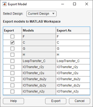
After designing a compensator, you can export it to the MATLAB workspace and create a model of the full closed-loop system. To export the tuned compensator:

In the app, select Export.
In the Export Model dialog box, select C, the compensator you designed, and click Export.

At the command line, enter the following command to create the closed-loop system, CL, from the open-loop transfer function, open_loopTF, and the compensator, C:

CL = feedback(C*open_loopTF,1)

The following model is returned:

CL =
 
                  -0.19414 (s-2)
  ----------------------------------------------
  (s^2 + 0.409s + 0.1136) (s^2 + 3.591s + 3.418)
 
Continuous-time zero/pole/gain model.

To create a step response plot of the closed-loop system, enter the following command.