segment
Piecewise distribution segments containing input values
Description
s = segment(pd,x)s of positive integers indicating which
segment in the piecewise distribution pd contains each quantile
value in x.
The values 1, 2, and 3 in s indicate the lower tail, center,
and upper tail segments in pd, respectively. If
pd does not include a lower tail segment, then 1 and 2
indicate the center and upper tail segments, respectively.
Examples
Generate a sample data set and create a paretotails object by fitting a piecewise distribution with Pareto tails to the generated data. Find the segment containing the specified quantile values by using the object function segment.
Generate a sample data set containing 20% outliers.
rng('default');  % For reproducibility
left_tail = -exprnd(1,100,1);
right_tail = exprnd(5,100,1);
center = randn(800,1);
x = [left_tail;center;right_tail];
Create a paretotails object by fitting a piecewise distribution to x. Specify the boundaries of the tails using the lower and upper tail cumulative probabilities so that a fitted object consists of the empirical distribution for the middle 80% of the data set and generalized Pareto distributions (GPDs) for the lower and upper 10% of the data set.
pd = paretotails(x,0.1,0.9)
pd =
Piecewise distribution with 3 segments
      -Inf < x < -1.33251    (0 < p < 0.1): lower tail, GPD(-0.0063504,0.567017)
   -1.33251 < x < 1.80149  (0.1 < p < 0.9): interpolated empirical cdf
        1.80149 < x < Inf    (0.9 < p < 1): upper tail, GPD(0.24874,3.00974)
Find the segment containing the specified points by using the segment function.
xpts = -3:3;
s = segment(pd,xpts)
s = 1×7

     1     1     2     2     2     3     3
1, 2, and 3 indicate the lower tail, center, and upper tail segments in pd, respectively.
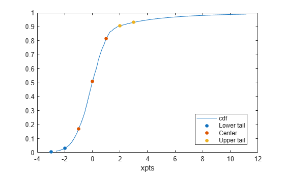
Draw the scatter plot of the points (xpts) grouped by their segments over the cumulative distribution function (cdf) plot. Plot the cdf of pd.
xgrid = linspace(icdf(pd,.01), icdf(pd,.99));
ygrid = cdf(pd,xgrid);
plot(xgrid,ygrid)
Superimpose the scatter plot of xpts by using gscatter.
hold on
gscatter(xpts,cdf(pd,xpts),s)
legend('cdf','Lower tail','Center','Upper tail')
hold off
Generate a sample data set and create a paretotails object by fitting a piecewise distribution with Pareto tails to the generated data. Find the segment containing the boundary points by using the object function segment.
Generate a sample data set containing 20% outliers.
rng('default');  % For reproducibility
left_tail = -exprnd(1,100,1);
right_tail = exprnd(5,100,1);
center = randn(800,1);
x = [left_tail;center;right_tail];
Create a paretotails object by fitting a piecewise distribution to x. Specify the boundaries of the tails using the lower and upper tail cumulative probabilities so that a fitted object consists of the empirical distribution for the middle 80% of the data set and generalized Pareto distributions (GPDs) for the lower and upper 10% of the data set.
pd = paretotails(x,0.1,0.9)
pd =
Piecewise distribution with 3 segments
      -Inf < x < -1.33251    (0 < p < 0.1): lower tail, GPD(-0.0063504,0.567017)
   -1.33251 < x < 1.80149  (0.1 < p < 0.9): interpolated empirical cdf
        1.80149 < x < Inf    (0.9 < p < 1): upper tail, GPD(0.24874,3.00974)
Return the boundary values between the piecewise segments by using the boundary function.
[p,q] = boundary(pd)
p = 2×1

    0.1000
    0.9000
q = 2×1

   -1.3325
    1.8015
The values in p are the cumulative probabilities at the boundaries, and the values in q are the corresponding quantiles.
Find the segment containing the boundary points by using the quantile values.
s1 = segment(pd,q)
s1 = 2×1

     2
     3
1, 2, and 3 indicate the lower tail, center, and upper tail segments in pd, respectively. The output s1 implies that the first boundary between the lower tail segment and the center segment belongs to the center segment, and the second boundary between the center segment and the upper tail segment belongs to the upper tail segment.
You can also use the cumulative probability values to find the corresponding segments.
s2 = segment(pd,[],[0;p;1])
s2 = 4×1

     1
     2
     3
     3
Input Arguments
Version History
Introduced in R2007a