Low Light Enhancement
This example shows how to enhance low-light images using an algorithm suitable for FPGAs.
Low-light enhancement (LLE) is a pre-processing step for applications in autonomous driving, scientific data capture, and general visual enhancement. Images captured in low-light and uneven brightness conditions have low dynamic range with high noise levels. These qualities can lead to degradation of the overall performance of computer vision algorithms that process such images. This algorithm improves the visibility of the underlying features in an image.
The example model includes a floating-point frame-based algorithm as a reference, a simplified implementation that reduces division operations, and a streaming fixed-point implementation of the simplified algorithm that is suitable for hardware.
LLE Algorithm
This example performs LLE by inverting an input image and then applying a de-haze algorithm on the inverted image. After inverting the low-light image, the pixels representing non-sky region have low intensities in at least one color channel. This characteristic is similar to an image captured in hazy weather conditions [1]. The intensity of these dark pixels is mainly due to scattering, or airlight, so they provide an accurate estimation of the haze effects. To improve the dark channel in an inverted low-light image, the algorithm modifies the airlight image based on the ambient light conditions. The airlight image is modified using the dark channel estimation and then refined with a smoothing filter. To avoid noise from over-enhancement, the example applies non-linear correction to better estimate the airlight map. Although this example differs in its approach, for a brief overview of low-light image enhancement, see Low-Light Image Enhancement (Image Processing Toolbox).
The LLE algorithm takes a 3-channel low-light RGB image as input. This figure shows the block diagram of the LLE Algorithm.
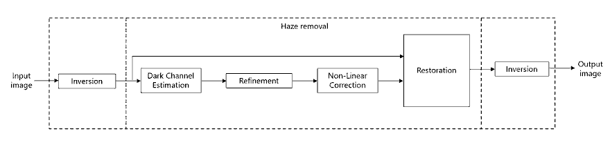
The algorithm consists of six stages.
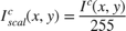
1. Scaling and Inversion: The input image ![$I^c(x,y), c\ \epsilon\ [r,g,b]$](../../examples/visionhdl/win64/LLEHDLExample_eq14214941893140577109.png) is converted to range [0,1] by dividing by 255 and then inverting pixel-wise.
is converted to range [0,1] by dividing by 255 and then inverting pixel-wise.

2. Dark Channel Estimation: The dark channel is estimated by finding the pixel-wise minimum across all three channels of the inverted image [2]. The minimum value is multiplied by a haze factor,  , that represents the amount of haze to remove. The value of is between 0 and 1. A higher value means more haze will be removed from the image.
![$$ I_{air}(x,y) = z \times \min_{c\ \epsilon\ [r,g,b]} I^c_{inv}(x,y)$$](../../examples/visionhdl/win64/LLEHDLExample_eq11388329026674567928.png)
3. Refinement: The airlight image from the previous stage is refined by iterative smoothing. This smoothing strengthens the details of the image after enhancement. This stage consists of five filter iterations with a 3-by-3 kernel for each stage. The refined image is stored in  . These equations derive the filter coefficients,
  , used for smoothing.
![$$I_{refined(n+1)}(x,y) = I_{refined(n)}(x,y) * h,\ n = [0,1,2,3,4]\ \& \ I_{refined(0)} = I_{air}$$](../../examples/visionhdl/win64/LLEHDLExample_eq16464911979157377608.png)
![$$ where \ h = \frac{1}{16} \left[ {\begin{array}{ccc} 1 & 2 & 1\\ 2 & 4 & 2\\ 1 & 2 & 1\\ \end{array} } \right] $$](../../examples/visionhdl/win64/LLEHDLExample_eq09179223797994285728.png)

4. Non-Linear Correction: To reduce over-enhancement, the refined image is corrected using a non-linear correction equation shown below. The constant,  , represents the mid-line of changing the dark regions of the airlight map from dark to bright values. The example uses an empirically-derived value of
  .
.
![$$ I_{nlc}(x,y) = \frac{[I_{refined}(x,y)]^4}{[I_{refined}(x,y)]^4+m^4} $$](../../examples/visionhdl/win64/LLEHDLExample_eq11708169642636935275.png)
5. Restoration: Restoration is performed pixel-wise across the three channels of the inverted and corrected image,  , as shown:
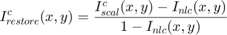
6. Inversion: To obtain the final enhanced image, this stage inverts the output of the restoration stage, and scales to the range [0,255].

LLE Algorithm Simplification
The scaling, non-linear correction, and restoration steps involve a divide operation which is not efficient to implement in hardware. To reduce the computation involved, the equations in the algorithm are simplified by substituting the result of one stage into the next stage. This substitution results in a single constant multiplication factor rather than several divides.
Dark channel estimation without scaling and inversion is given by
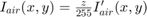 where
where ![$I'_{air}(x,y) = 255 - \min_{c\ \epsilon\ [r,g,b]}I^c(x,y)$](../../examples/visionhdl/win64/LLEHDLExample_eq07345798975282197167.png)
The result of the iterative refinement operation on  is
is
where
![$$I'_{refined(n+1)}(x,y) = I'_{refined(n)}(x,y) * h,\ n = [0,1,2,3,4]\ \& \ I'_{refined(0)}(x,y) = I'_{air}(x,y)$$](../../examples/visionhdl/win64/LLEHDLExample_eq13349115930010945499.png)
Substituting  into the non-linear correction equation gives
![$$I_{nlc}(x,y) = \frac{z^4[I'_{refined}(x,y)]^4}{z^4[I'_{refined}(x,y)]^4 + (255 \times m)^4}$$](../../examples/visionhdl/win64/LLEHDLExample_eq04292894015724166447.png)
Substituting into the restoration equation gives
![$$I^c_{restore}(x,y) = 1 - \frac{I^c(x,y)}{255} - \frac{I^c(x,y)}{255}\frac{z^4}{(255 \times m)^4}[I'_{refined}(x,y)]^4$$](../../examples/visionhdl/win64/LLEHDLExample_eq09542056517844570922.png)
Subtracting  from 1 and multiplying by 255 gives
![$$I^c_{enhanced}(x,y) = I^c(x,y)\times \left(1 + \Big[\frac{z}{255 \times m}I'_{refined}(x,y)\Big]^4\right)$$](../../examples/visionhdl/win64/LLEHDLExample_eq03333235659495581719.png)
With the intensity midpoint, , set to 0.6 and the haze factor, , set to 0.9, the simplified equation is
![$$ I^c_{enhanced}(x,y) = I^c(x,y) \times \left( 1 + \Big[\frac{1}{170}I'_{refined}(x,y)\Big]^4 \right)$$](../../examples/visionhdl/win64/LLEHDLExample_eq02875608894175652083.png)
In the equation above, the factor multiplied with  can be called the Enhancement Factor. The constant
  can be implemented as a constant multiplication rather than a divide. Therefore, the HDL implementation of this equation does not require a division block.
HDL Implementation
The simplified equation is implemented for HDL code generation by converting to a streaming video interface and using fixed-point data types. The serial interface mimics a real video system and is efficient for hardware designs because less memory is required to store pixel data for computation. The serial interface also allows the design to operate independently of image size and format, and makes it more resilient to video timing errors. Fixed-point data types use fewer resources and give better performance on FPGA than floating-point types.
open_system('LLEExample');
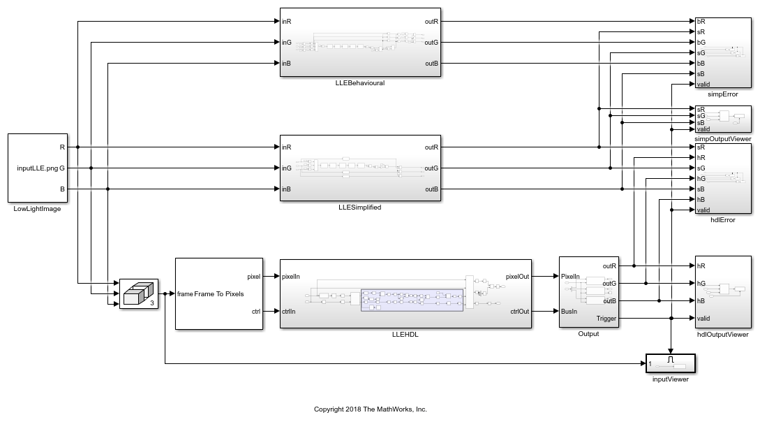
The location of the input image is specified in the LowLightImage block. The LLEBehavioural subsystem computes the enhanced image using the raw equations as described in the LLE Algorithm section. The LLESimplified subsystem computes the enhanced image using the simplified equations. The simpOutputViewer shows the output of the LLESimplified subsystem.
The LLEHDL subsystem implements the simplified equation using a streaming pixel format and fixed-point blocks from Vision HDL Toolbox™. The Input subsystem converts the input frames to a pixel stream of uint8 values and a pixelcontrol bus using the Frame To Pixel block. The Output subsystem converts the output pixel stream back to image frames for each channel using the Pixel To Frame block. The resulting frames are compared with result of the LLESimplified subsystem. The hdlOutputViewer subsystem and inputViewer subsystem show the enhanced output image and the low-light input image, respectively.
open_system('LLEExample/LLEHDL');

The LLEHDL subsystem inverts the input uint8 pixel stream by subtracting each pixel from 255. Then the DarkChannel subsystem calculates the dark channel intensity minimum across all three channels. The IterativeFilter subsystem smooths the airlight image using sequential Image Filter blocks. The bit growth of each filter stage is maintained to preserve the precision. The Enhancement Factor is calculated in EnhancementFactor area. The constant is implemented using Constant and Reciprocal blocks. The Pixel Stream Aligner block aligns the input pixel stream with the pipelined, modified stream. The aligned input stream is then multiplied by the modified pixel stream.
Simulation and Results
The input to the model is provided in the LowLightImage (Image From File) block. This example uses a 720-by-576 pixel input image with RGB channels. Both the input pixels and the enhanced output pixels use uint8 data type. The necessary variables for the example are initialized in PostLoadFcn callback.
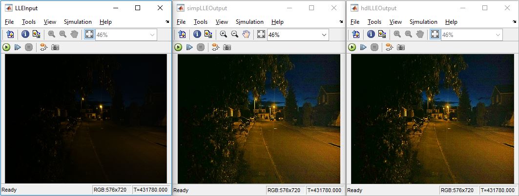
The LLEBehavioural subsystem uses floating-point Simulink blocks to prototype the equations mentioned in the LLE Algorithm section. The LLESimplified subsystem implements the simplified equation in floating-point blocks, with no divide operation. The LLEHDL subsystem implements the simplified equation using fixed-point blocks and streaming video interface. The figure shows the input image and the enhanced output images obtained from the LLESimplified subsystem and the LLEHDL subsystem.
The accuracy of the result can be calculated using the percentage of error pixels. To compute the percentage of error pixels in the output image, the difference between the pixel value of the reference output image and the LLEHDL output image should not be greater than one, for each channel. The percent of pixel values that differ by more than 1 is computed for the three channels. The simpError subsystem compares the result of the LLEBehavioural subsystem with the result of the LLESimplified subsystem. The hdlError subsystem compares the result of the LLEHDL subsystem with the result of the LLESimplified subsystem. The error pixel count is displayed for each channel. The table shows the percentage of error pixels calculated by both comparisons.
![]()
References
[1] X. Dong, G. Wang, Y. Pang, W. Li, and J. Wen, "Fast efficient algorithm for enhancement of low lighting video" IEEE International Conference on Multimedia and Expo, 2011.