Triggered Capture Using Energy Detection

This example shows how to use a software-defined-radio (SDR) to capture data from the air using energy detection. The example also shows how to use the transmit capabilities of the same radio to loop back a test waveform.

Set Up Radio

Call the radioConfigurations function. The function returns all available radio setup configurations that you saved using the Radio Setup wizard.

savedRadioConfigurations = radioConfigurations;

To update the dropdown menu with your saved radio setup configuration names, click Update. Then select the radio to use with this example.

savedRadioConfigurationNames = [string({savedRadioConfigurations.Name})];
radio = savedRadioConfigurationNames(1) ;

Generate Transmission Waveform

Create a transmission waveform containing a chirp signal with zero padding to simulate a radar impulse signal.

chirpSignal = single(chirp(0:1/1e3:2,0,0.5,15,'complex')).';
chirpSignal(end) = [];  % removing the last sample of the chirp signal so that is an even length
PadLen = 6500;
zeroSignal = complex(zeros(PadLen,1),zeros(PadLen,1));
inputSignal = [zeroSignal; chirpSignal*0.999; zeroSignal];

Plot transmission waveform.

figure();
subplot(2,1,1); plot(real(inputSignal));
subtitle("Real Part");
xlabel("Samples"); 
ylabel("Amplitude");
title("Waveform with Chirp Signal");
subplot(2,1,2); 
plot(imag(inputSignal),Color='r');    
subtitle("Imaginary Part"); 
xlabel("Samples"); 
ylabel("Amplitude");

Configure Energy Detector

Create an energy detector object with the specified radio. Because the object requires exclusive access to radio hardware resources, before running this example for the first time, clear any other object associated with the specified radio. To speed up the execution of the example in subsequent runs, reuse your new workspace object.

if ~exist("ed","var")
    ed = energyDetector(radio);
end

Set the RF properties of the energy detector. Set the RadioGain property according to the local wireless channel.

ed.SampleRate = 30720000;
ed.CenterFrequency = 2450000000;
ed.RadioGain = 30; % Try to increase if signal levels are low until detection is successful

To update the dropdown menu with the antennas available for capture on your radio, call the hCaptureAntennas helper function. Then select the antenna to use with this example.

captureAntennaSelection = hCaptureAntennas(radio);
ed.Antennas = captureAntennaSelection(2);

Set the capture data type to the data type of the generated transmission waveform.

ed.CaptureDataType = "single";

Configure Transmission Variables

Set the transmit gain and transmit antenna values. Set the transmit gain variable according to the local wireless channel.

txGain = 30; % Try to increase if signal levels are low until detection is successful

To update the dropdown menu with the antennas available for transmit on your radio, call the hTransmitAntennas helper function. Then select the antenna to use with this example.

transmitAntennaSelection = hTransmitAntennas(radio);
txAntenna = transmitAntennaSelection(2); 

Detect Energy Signal Using Fixed Threshold and Capture Data

To capture data when signal energy is greater than a fixed threshold, set the threshold method of the energy detector to "fixed". By then setting the fixed threshold to 0, you can analyze the behavior of the energy detector and understand how to set the fixed threshold value for successful detection. These settings also help you understand how to set the minimum threshold in adaptive threshold mode.

To set the threshold method, you must first stop any ongoing transmission by calling the stopTransmission function on the energy detector object. Set the energy detector to use fixed threshold.

ed.ThresholdMethod = "fixed";

Set the fixed threshold initially to 0.

ed.FixedThreshold = 0;

Set the sliding window length to 300 samples. The optimal window length depends on the signal you are detecting and the channel quality.

ed.WindowLength = 300;  % Try to increase if signal levels are low until detection is successful

Transmit the test waveform.

transmit(ed,inputSignal,"continuous",TransmitGain=txGain, ...
    TransmitCenterFrequency=ed.CenterFrequency,TransmitAntennas=txAntenna);

Use the plotDetectionSignals function to analyze the behavior of the detector by plotting 50,000 samples. Because the fixed threshold value is 0, the possible detection area, highlighted in green, includes all samples.

plotDetectionSignals(ed,5e4);

In fixed mode, a capture triggers if the integrated signal energy is higher than the energy threshold.

Choose a threshold value that is above the noise floor and below the peak magnitude of the signal. Plot the threshold information again and confirm that the trigger point occurs where signal energy is present. Adjust and plot again until you are satisfied with the output.

ed.FixedThreshold = 4;
plotDetectionSignals(ed,5e4);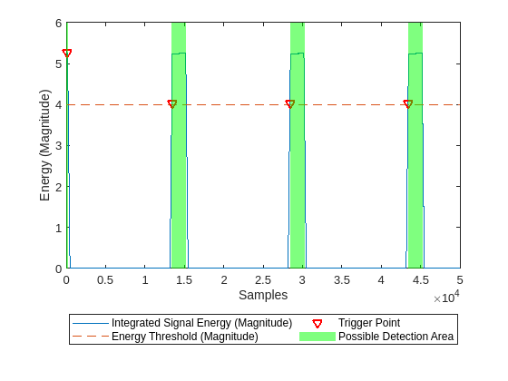

Once the threshold is set, capture data.

[data, ~, ~, status] = capture(ed,3e3,seconds(1));

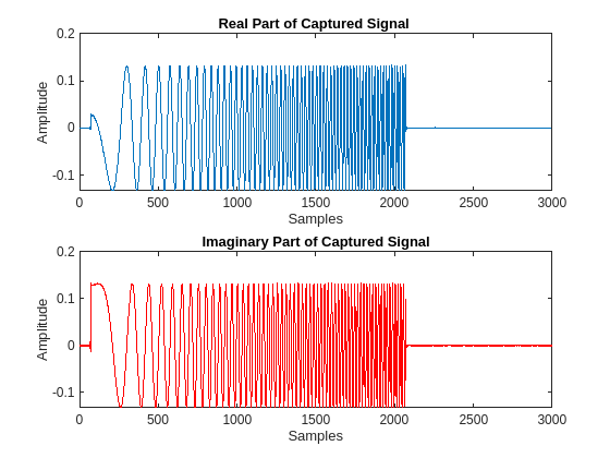
Use the hPlotCapturedData helper function to plot the captured signal.

hPlotCapturedData(data,status);

ed.stopTransmission;

Detect Energy Signal Using Adaptive Threshold and Capture Data

As an alternative to using the fixed threshold, you can trigger data capture when energy increases abruptly in the channel. This method can be configured to ensure that noise variations do not cause a trigger point. By setting the energy delta threshold and minimum energy to 0, you can analyze the behavior of the energy detector and understand how to configure the adaptive threshold for successful detection.

To set the threshold method, you must first stop any ongoing transmission by calling the stopTransmission function on the energy detector object. Set the energy detector to use adaptive threshold.

ed.stopTransmission;
ed.ThresholdMethod = 'adaptive';

Set the energy delta threshold to 0 dB and minimum energy value to 0.

ed.EnergyDeltaThreshold = 0;
ed.MinimumEnergy = 0; 

Transmit the test waveform.

transmit(ed,inputSignal,"continuous",TransmitGain=txGain, ...
    TransmitCenterFrequency=ed.CenterFrequency,TransmitAntennas=txAntenna);

Use the plotDetectionSignals function to analyze the behavior of the detector by plotting 50,000 samples. Adjust the thresholds if necessary.

plotDetectionSignals(ed,5e4);

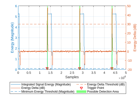
In adaptive threshold mode, a capture triggers if both the energy delta and integrated signal energy are higher than the energy delta threshold and minimum energy threshold respectively.

To remove the trigger points when the integrated signal energy is near zero, set the minimum energy to a value that is above the noise floor. Adjust the energy delta threshold and plot the threshold information repeatedly until the trigger points occur at the desired location.

ed.EnergyDeltaThreshold = 30; % dB
ed.MinimumEnergy = 0.1;
plotDetectionSignals(ed,5e4);

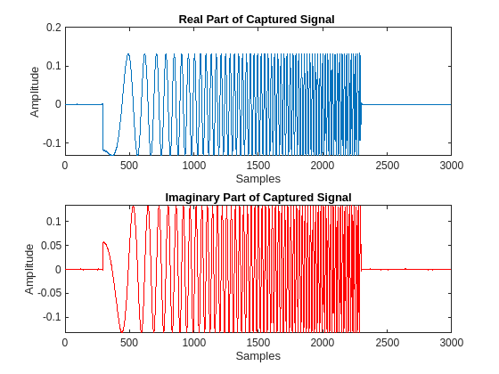
Once the threshold is configured, capture data and plot the captured signal.

[data, ~, ~, status] = capture(ed,3e3,seconds(1));
hPlotCapturedData(data,status);

Detect Multiple Consecutive Signals

You can perform multiple consecutive energy detections by setting the NumCaptures property to a value greater than 1. Set the NumCaptures property to 3 to capture three consecutive signals using the same adaptive thresholding criteria. Then, use the hPlotCapturedData helper function to plot the captured signals.

[data, timestamps, ~, status] = capture(ed, 3e3, seconds, NumCaptures = 3);
hPlotCapturedData(data, status);

Display the time stamp for each capture. These are returned in datetime format to nanosecond precision.

disp(timestamps);

   01-Nov-2023 14:08:06.340028527
   01-Nov-2023 14:08:06.340516808
   01-Nov-2023 14:08:06.341005089

Tune Window Length to Balance Precision and Stability

Reduce the window length to 15 to increase the sensitivity.

ed.WindowLength = 15;
ed.EnergyDeltaThreshold = 30; % dB
ed.MinimumEnergy = 0.1;
ed.TriggerOffset = 0;
plotDetectionSignals(ed,5e4);

[data, ~, ~, status] = capture(ed,3e3,seconds(1));
hPlotCapturedData(data,status);

Using a shorter window length will allow you to start your capture more precisely at the start of the signal. However, it also increases the sensitivity of the detector, so you might need to recalibrate the thresholds.

Set Trigger Offset

To capture data before the trigger point, set the trigger offset to 3000 samples.

ed.stopTransmission;
ed.TriggerOffset = -3000;

Transmit the test waveform, capture data, and plot.

transmit(ed, inputSignal,"continuous",TransmitGain=txGain, ...
    TransmitCenterFrequency=ed.CenterFrequency,TransmitAntennas=txAntenna);
% Detect and capture 5000 samples, with a 1 second timeout
[data, ~, ~, status] = capture(ed,5e3,seconds(1));
hPlotCapturedData(data,status);

To end the continuous transmission, call the stopTransmission function on the energy detector object.

ed.stopTransmission;