Mettiti comodo!
Discussions è il tuo spazio in cui puoi conoscere i tuoi colleghi, affrontare insieme le sfide più grandi e divertirti.
- Vuoi vedere gli ultimi aggiornamenti? Segui i punti salienti!
- Cerchi tecniche per migliorare le tue competenze in MATLAB o Simulink? Tips & Tricks è la soluzione che fa per te!
- Vuoi condividere la barzelletta, il gioco di parole o il meme matematico perfetto? Non cercare altro che il divertimento!
- Pensi che ci sia un canale di cui abbiamo bisogno? Raccontaci di più in Ideas
Discussions aggiornate

What does the participation matrix represent - from the Modern Grid Stability with IBRs: Leveraging Simulation and Control Design session.

Currently, MathWorks provides free access to MATLAB Online for anyone with a personal account. Each account receives 20 hours of usage per month and includes access to the following 10 toolboxes:
- Control System Toolbox(控制系统工具箱)
- Curve Fitting Toolbox(曲线拟合工具箱)
- Deep Learning Toolbox(深度学习工具箱)
- Image Processing Toolbox(图像处理工具箱)
- Optimization Toolbox(优化工具箱)
- Signal Processing Toolbox(信号处理工具箱)
- Statistics and Machine Learning Toolbox(统计与机器学习工具箱)
- Symbolic Math Toolbox(符号数学工具箱)
- Text Analytics Toolbox(文本分析工具箱)
I would like to know whether it is possible to customise the selection of these 10 toolboxes. For example, I mainly work in computer vision, but Computer Vision Toolbox is not included in the current offering, which is quite disappointing because I cannot use it.
At the same time, several of the included toolboxes are not useful for my work, such as Control System Toolbox and Signal Processing Toolbox. Therefore, it would be great if users could choose the toolboxes that best fit their needs rather than being limited to a fixed set of toolboxes.

FOLD: One Button, Two Worlds
For the MATLAB One-Button Game Mini Hack, I developed FOLD, a six-level puzzle-platformer built entirely in MATLAB.
Unlike traditional platformers, the player does not directly control the character. Instead, the character moves automatically, while a single button changes the geometry of the environment.
Each press rotates platforms, changes available paths, and activates or deactivates obstacles.
Play FOLD here:
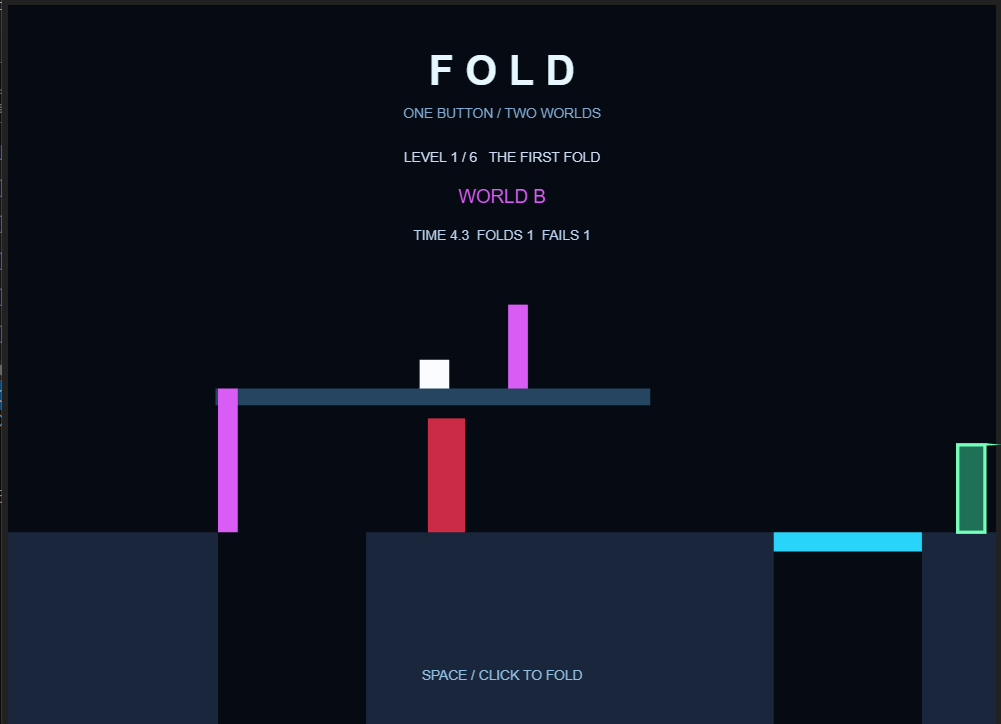
FOLD — Rotating platforms and phase-based obstacles controlled with a single button.
1. Creating Rotating Platforms with Trigonometry
One of the main technical challenges was creating platforms that rotate around a fixed pivot.
Rather than recreating graphical objects every frame, I calculate the vertices of each platform using trigonometric functions.
For a platform with length L, thickness w, and rotation angle a:
dx=L*cos(a);
dy=-L*sin(a);
nx=w*sin(a);
ny=w*cos(a);
px=[x x+dx x+dx+nx x+nx];
py=[y y+dy y+dy+ny y+ny];
These coordinates define the four corners of the platform.
By updating the XData and YData properties of an existing patch, MATLAB can animate the platform without creating new graphics objects every frame.
This approach keeps the animation simple and efficient.
2. Making the Character Move with a Platform
Initially, the character would fall whenever a platform started rotating.
To solve this, I introduced a mechanism that temporarily attaches the character to the rotating platform.
The character's position is calculated relative to the platform's pivot:
s.x=170+s.dist*cos(a)-12;
s.y=440-s.dist*sin(a)-24;
Here, s.dist represents the distance along the platform, while a is the current rotation angle.
This allows the character to move together with the platform and reach elevated sections of the level.
3. Designing Gameplay Around a Single Button
The most interesting design challenge was creating meaningful gameplay with only one input.
FOLD uses two world states: A and B.
Pressing SPACE or clicking the mouse switches between these states. Multiple platforms respond simultaneously, while certain obstacles become active or inactive.
This creates situations where opening one path may close another.
Across six levels, players must learn to anticipate how their actions affect the environment.
The objective was to make the game progressively more strategic without introducing additional controls.
4. Optimizing MATLAB Code for the Character Limit
The competition limits submissions to 10,000 characters.
One important discovery was that the validator's character count could differ significantly from the raw source file length.
Removing whitespace alone was not sufficient.
I reduced code duplication, reused helper functions, represented level configurations using arrays, and simplified unnecessary graphical elements.
The final implementation successfully passed minihackContest.validate.
5. What I Learned
Developing FOLD helped me explore several useful MATLAB techniques:
- Updating existing graphical objects instead of recreating them.
- Applying trigonometry to interactive 2D geometry.
- Managing game states and frame-based updates.
- Designing multiple puzzles around a single input.
- Optimizing code under strict technical constraints.
AI assistance was used during prototyping, debugging, and code refinement. The gameplay was tested locally in MATLAB, and the final submission passed the official contest validator.
The main takeaway: limitations can encourage creativity. With a single button, basic trigonometry, and carefully designed state transitions, it is possible to build an interactive puzzle game with surprisingly varied gameplay.

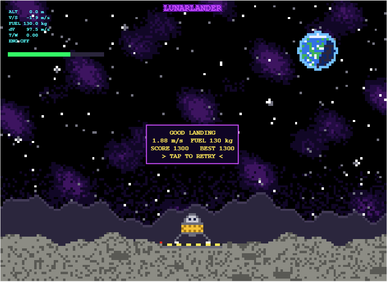
My entry for the one-button game mini hack Lunar Lander - Tap to Burn, is a one-button powered descent. You start 500 m above the surface, falling at 10 m/s, with 200 kg of propellant. One tap turns on the engine, and the next tap stops it.
How scoring works
- Crash: landing at 3 m/s or faster scores 0.
- Abort: rising above 750 m scores 0.
- Safe landing: below 3 m/s scores 10 points per kilogram of fuel remaining.
- Perfect touchdown: below 1 m/s doubles the reward to 20 points per kilogram of fuel remaining.
Physics in the game
- Fuel mass decreases as propellant is burned.
- Gravity continuously accelerates the lander downward.
- The engine does not reach full thrust instantly, so timing matters.
- The display turning red indicates when a full thrust landing burn becomes possible.
Display readouts
- ALT [m]: Height above the surface.
- V/S [m/s]: Vertical speed.
- FUEL [kg]: Remaining propellant.
- dV [m/s]: remaining velocity change the fuel can provide, from the rocket equation Δv=Isp·g₀·ln(m/m_dry).
- T/W: Thrust to weight ratio.
My best so far is 1300. Has anyone managed a sub 1m/s landing?

I thought I had the game in pretty good shape until I tried it in MATLAB Online. A launch that felt immediate on desktop could feel slower in the browser, which matters in a game where timing is the main control.
I built Slingshot Home: Escape Saturn for the MATLAB One-Button Game Mini Hack. The goal is to time your launches to travel between 15 of Saturn’s moons and return to Earth, with three shields and a clock counting down.
Getting the game to feel responsive took a few iterations, particularly when running it in MATLAB Online. Here are some of the approaches that worked well.
Reuse Graphics Objects
The game creates 21 graphics objects during initialization and reuses them throughout gameplay. Instead of recreating the scene, it updates properties such as position, color, and text.
I also check whether a property has changed before assigning it again. Static planets and labels do not need to be updated as frequently as the spacecraft.
For the Mini Hack, the game harness handles the window, input, and drawing loop. The game provides the init, update, and render functions.
Use Elapsed Time for Motion
The spacecraft moves around each moon using basic trigonometry:
theta = startAngle + angularSpeed*elapsedTime;
position = moonCenter + radius*[cos(theta), sin(theta)];
heading = [-sin(theta), cos(theta)];
Pressing the button launches the spacecraft along the tangent to its current orbit, so the gameplay is based on timing rather than steering.
Calculating the orbital angle from elapsed game time, rather than advancing it by a fixed amount per frame, also makes the motion less dependent on rendering speed.
Separate Trajectory Calculation from Rendering
I used ode45 to calculate each flight trajectory, then deval and interpolation to provide positions during playback. This avoids solving the trajectory again on every frame.
The physics is intentionally simplified. The moons remain in fixed positions, captures are assisted, and the escape gate represents leaving Saturn’s sphere of influence rather than calculating its actual boundary. These assumptions are documented in the code comments.
Generate Textures in MATLAB
The planet textures are generated directly in MATLAB, so there are no external image files to load:
MATLAB
x = linspace(-1,1,80);
z = max(0,1-x.^2-x'.^2);
brightness = max(.1,.8*sqrt(z)-.6*x);
This produces directional lighting while retaining some brightness on the night side. The textures are generated once during initialization.
Increasing the texture resolution helped smooth the edges, but adjusting the lighting had a larger effect on the overall appearance.
Test as You Go
I used Codex to help edit and refine the code. Through MATLAB MCP, it could run MATLAB code, inspect Code Analyzer results, and exercise states such as countdown, launch, and restart.
That was useful for finding issues, but running and playing the game was still important. Some things only became apparent during gameplay, such as a launch feeling delayed or an orbit being difficult to see. I also tested regularly in MATLAB Online rather than relying only on desktop behavior.
I used the Mini Hack validator to keep track of the character limit:
minihackContest.validate
The validator count differs from the raw file size. Comments are excluded, so I could document the physics and assumptions without using the executable-code budget.
Try It in MATLAB Online
One feature I liked about the final result is that there is very little setup required to try it.
Click “Play game,” then “Run this app,” and the game runs in the browser.
For me, the biggest improvements came from fairly small changes: reusing graphics objects, basing motion on elapsed time, calculating trajectories separately from rendering, and testing regularly in MATLAB Online.

My second entry, Event Horizon (entry 16546), puts you in orbit around a black hole. Tapping fires your engine and climbs, and the accretion disk's drag pulls you down. Lower orbits slow your clock, so your score is how many years into Earth's future you travel. Flares light up rings of the disk, and you have to get out of a red band before it turns white and burns.
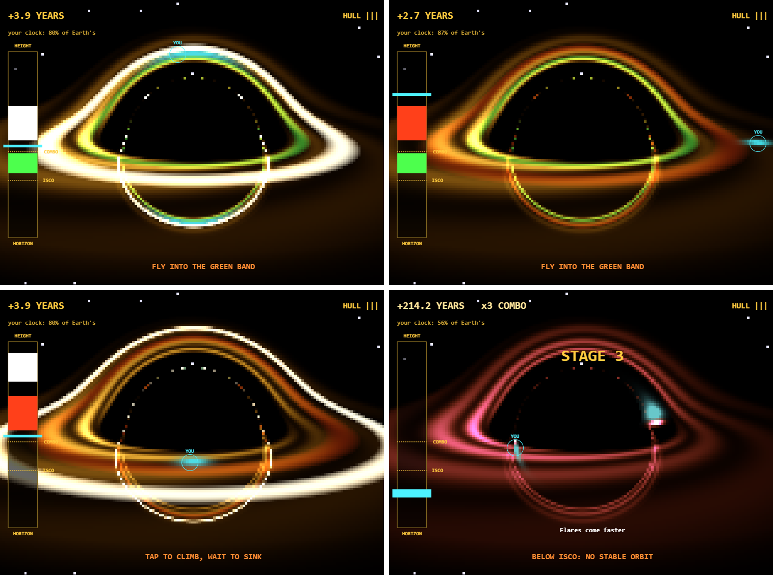
Real frames from the game. In the top left, the ship (cyan, marked YOU) is behind the hole, and gravity bends its light into an arc over the top.
The picture isn't drawn by hand. It comes from tracing light through the Schwarzschild metric, the spacetime around a non-spinning black hole. Here is what I learned building it, again with help from an AI coding assistant (Claude Code), testing each change in MATLAB.
1. Trace the light once, then shade the map every frame
My first prototype traced one light ray per pixel every frame. With rays bending around the hole, that took about 240 ms per frame at 160 by 120 pixels, far over the 33 ms a 30 fps frame allows.
The fix was to notice that the camera never moves. Each pixel's ray always lands in the same place, so I trace every ray once in init and store where it crosses the plane of the disk. In these units, with the Schwarzschild radius set to 1, a light ray's path follows a simple force law, which I step for all 19,200 rays at once:
h2 = sum(cross(P,V).^2); % each ray's angular momentum squared
for k = 1:150
d = min(.07*vecnorm(P),1); % smaller steps near the hole
Q = P+V.*d;
V = V-1.5*h2.*Q./vecnorm(Q).^5.*d;
% ...record where each ray crosses z = 0, drop rays that escape or fall in
end
Each ray keeps its first two crossings of the disk plane. The first is the direct view. The second is light that went around the back of the hole, which is why you can see the far side of the disk both above and below the shadow.
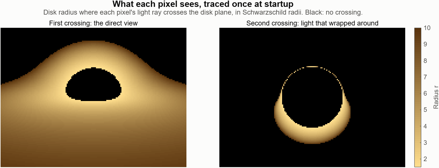
The trace takes about 160 ms at startup on my PC. After that, each frame only shades the stored points, and the game's whole frame work is about 6 ms.
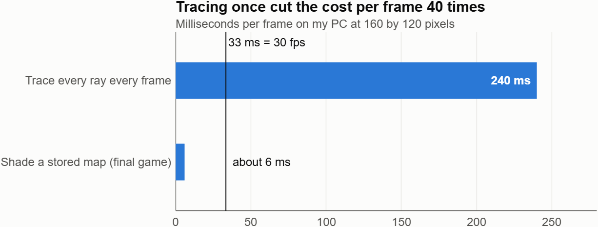
The 240 ms comes from an early prototype with a slightly different camera, so treat the ratio as approximate.2. Paint the game into the disk, and gravity bends it for free
Because the map stores a disk position for every pixel, anything I draw in disk coordinates gets lensed automatically. The ship is just a glow centered on its position in the disk, and the flares are rings of disk radius:
zs = s.r*exp(1i*s.ph); % ship position as x + iy
S(L.i) = S(L.i)+exp(-abs(L.c-zs).^2/.2); % L.c: disk point of each pixel
b = max(0,1-((L.r-s.fc)./s.fw).^2); % flare rings by radius
When the ship passes behind the hole, its image smears into arcs above and below the shadow. No extra code does that. The engine exhaust from each tap is drawn the same way, so it bends too.
Storing disk points as complex numbers kept the distance check to one short line.
3. Real physics needed a real gauge
The orbit uses the Schwarzschild radial equation, so the innermost stable orbit at r = 3 is real: below it, no orbit is stable and the ship slides inward. Time dilation sets the score. A circular orbit's clock runs at sqrt(1 - 1.5/r) of a distant clock, so Earth gains the rest:
s.vr = s.vr+(-.5/s.r^2+s.L^2/s.r^3-1.5*s.L^2/s.r^4-.04*s.vr)*T;
s.yrs = s.yrs+10*h*s.m*(1-sqrt(max(0,1-1.5/s.r)));
The physics made two first designs fail:
- Head-on debris didn't work. Moving up or down is slower than going around the hole, so you met debris before a burn could lift you clear. Climbing one unit took about 3 s even tapping 5 times a second. I replaced debris with flares that warn for 3.5 s, and I sped up game time 1.6 times.
- A beautiful view isn't a readable one. In my first playtest, I couldn't tell what a tap did, because the lensed ship jumps around the screen. A simple height gauge on the left fixed that. Tapping moves your bar up, red bands are flares, and green bands are bonuses. The black hole is the show, and the gauge is the controller.
After that came the parts that made it fun: a combo multiplier for staying deep, stages every 100 years with faster and drifting flares, and a close-call bonus for clearing a flare by a hair.4. Small tricks that saved characters
The final file counts 9,993 of 10,000 characters. The counter reformats your code first, so comments are free but spaces and indentation count, as I described in my first post. These helped:
- Divide by zero to hide things. 0/0 is NaN, and graphics skip NaN points, so one expression both positions and hides a marker:G.gs.YData = [1 1]*(100+60*(s.r-1))+0/(s.mode == 1);
- Make several texts in one call. text takes vectors and a cell array of strings:text(ax,[103 108 50 50],[220 280 88 502],{'ISCO','COMBO','HORIZON','HEIGHT'},f{:});
- Store end times, not countdowns. A message that shows until s.t < s.got needs no line to count it down each frame.
- Write constants out when they're fixed. My camera never moves, so its right and up vectors became constants instead of cross products.
One trim I had to undo: dropping a normalization in the star placement put stars inside the black hole's shadow. Look at the frames after every trim.Play it
If MATLAB Online is slow for you, run it in desktop MATLAB: download the starter project, copy the entry's code into game.m, and run minihackContest.play.
How many years into the future can you get?

A huge thank you to everyone who participated in the MATLAB STEM Showcase!
What makes these contributions especially meaningful is that their impact doesn’t end with the contest. Your work can continue to help students, educators, engineers, scientists, and curious learners explore STEM concepts for years to come.
And now, it’s time to celebrate our winners!
🥇 STEM Domain Awards
Congratulations to our STEM Domain Award winners. Each of you will receive a $50 Amazon gift card.
AI & Data Science:
@Yiheng for Inside the VAE
Physics:
Mathematics:
Engineering:
Life Sciences:
Earth & Climate Science:
🎁 Weekly Prize Winners
Congratulations as well to all of our Weekly Prize winners! You will receive a MathWorks T-shirt or a pair of socks.
@Anshika, @Jan Studnicka, @Michelle, @Abhishek, @Dr. Mishaal A. AbdulKareem, @Harshad, @KARUPPASAMYPANDIYAN M, @Umar, @Heze Chen, @Jamil Kasan, @Jorge Paloschi, @Pauli Huusari, @Rodolfo
Congratulations to all our winners, and thank you again to everyone who participated!
We hope you’ll continue creating, exploring, and sharing interactive STEM experiences with the MATLAB community.

Lira vanished 19 years ago. Now her signal is back. You control a radio telescope that sweeps the sky, and you only have one button (SPACE or click).
- Watch the dish sweep left and right. When the beam passes over a “?” in the sky, press to lock onto the signal.
- Then tap as fast as you can to collect pulses (up to 8 in 2.4 seconds).
- Each signal turns out to be an ALIEN, a NEW PLANET or a BLACK HOLE, and a little face appears in the sky.
- Lira’s signature is SHORT-SHORT-LONG. Aliens repeat it, so they need more pulses to be confirmed. If you don’t reach the goal, the alien gets away and you can try again.
- Every alien you confirm decodes part of a hidden message. Clear the three sectors (Pulsar, Dust Cloud, Deep Space) to read it.
HOW THE CODE WORKS
The game follows the contest contract: game() returns init, update and render.
1. init – builds everything once.
It draws the pixel-art backdrop (one small image with a sunset in color bands), the dish, the wave panel, the texts and the three faces. Each face is a few ellipse patches inside an hggroup, parented to an hgtransform so it can be moved and scaled later.
2. update – the game logic.
The game is a small state machine with one phase number: 0 ready, 1 scan, 2 collect, 3 transit, 4 done. The same button means “start”, “lock on” or “tap fast” depending on the phase. A short cooldown after each press avoids double hits.
The dish angle is a triangle wave over time:
a = 110*(1-abs(mod(t*rate/110,2)-1))-55
A target can be locked when it is within 14 degrees of the beam. Each sector raises the sweep rate.
3. Signals and their type.
Each signal is built from two 3-letter patterns of short (S) and long (L) pulses, drawn as one waveform. The type comes straight from the patterns:
- both halves equal to Lira’s SSL → alien
- both halves equal but different → new planet
- halves different → black hole
So the wave you see on screen really tells you what you found.
4. render – only updates properties.
Nothing is created while playing. Each frame only changes XData/YData of the dish and wave, the String and Color of the texts, and the Matrix of each face (makehgtform with translate and scale). The faces “pop” on every tap with a simple scale change. This keeps the game smooth.
5. Fitting under 10,000 characters.
The validator counted more than the file size, so I used anonymous helpers for repeated line/text calls, stored shapes in small matrices and ran minihackContest.validate often.
Thanks for playing, and good luck everyone!

Thanks to Dr. Riyadh Kenaya and Arnie Berlin for the session and for answering my questions live: UE5 handles radial and tangential distortion, rolling shutter would be added in Simulink, and the synthetic data is meant for design of experiments on extrinsic limits rather than exact calibration.
A few follow-ups:
- The demo results showed a mean calibration error of 3.85 px, with camera 1 at 7.33 px. On synthetic images where the true intrinsics are known, what drives that error: the distortion model fit, board detection near the image edges, or something else?
- Can the ChArUco board poses be set from a script instead of the Control Center sliders? That would let a calibration campaign run as a Monte Carlo sweep over board placement and lighting.
- Does the camera model support fisheye or rational distortion models for wide lenses (around 100 degrees horizontal)?
- With a 32-channel lidar, only a few rings hit each board. How much does camera-to-lidar extrinsic accuracy degrade as the boards move farther away?
I would also be glad to try the example if the code is available.
Thanks to Siddharth Jawahar for the Misconceptions in Control Design workshop. I worked through the M3 to M5 models and have three follow-ups.
- Transport delay in PID Tuner. In M5, the tuned design showed 60 degrees of phase margin at 5.27 rad/s, while the gain margin sat at 25 rad/s for both the original and the tuned gains. That suggests the transport delay sets the phase crossover. Does PID Tuner linearize the Transport Delay block exactly, use a Pade approximation, or tune on the delay-free plant? If it drops the delay, the margins on screen would be optimistic.
- Missing the settling spec. The tuned design settled in 1.02 s against the 0.8 s requirement, while rise time and overshoot passed. Which would you trade first: a little more overshoot, derivative action, or reducing the delay itself?
- Windup in field logs. The M4 hand-built PI asked for about 26 V against a 12 V driver limit and overshot by 187.7 percent after the disturbance cleared. On real hardware, is the requested voltage pinned at the limit while the error keeps growing the signature you look for? Do you recommend logging requested and applied voltage as separate signals by default?
Context: I work on simulation validation and am building a fault-injection testbed for a small robot that injects latency, jitter, and packet loss on the control link. Variable delay is the case I care about most, so any pointers on modeling jitter (for example with the NetworkCondition block) would help.
Thanks!
In our previous Mini Hack contests, you amazed us with creative images, animations, and videos. This year, we’re trying something new: Let’s make games!
With the help of Agentic AI, you don’t have to write all the code yourself. Bring your idea, and creativity, then work with AI to turn it into a MATLAB game.
New to Agentic AI? No problem!
We’ve created a step-by-step tutorial that can help you set up the MATLAB Agentic AI workflow in about 20 minutes, including a video to walk you through the process. This contest is about learning while having fun. We want you to experience the MATLAB Agentic AI workflow by actually using it to build something.
And don’t just create; share what you learn! Create a Tips & Tricks post to share your Agentic AI experience, discoveries, and useful tips with the community.
So get set up, start experimenting, have fun creating, and win big prizes! 🎁
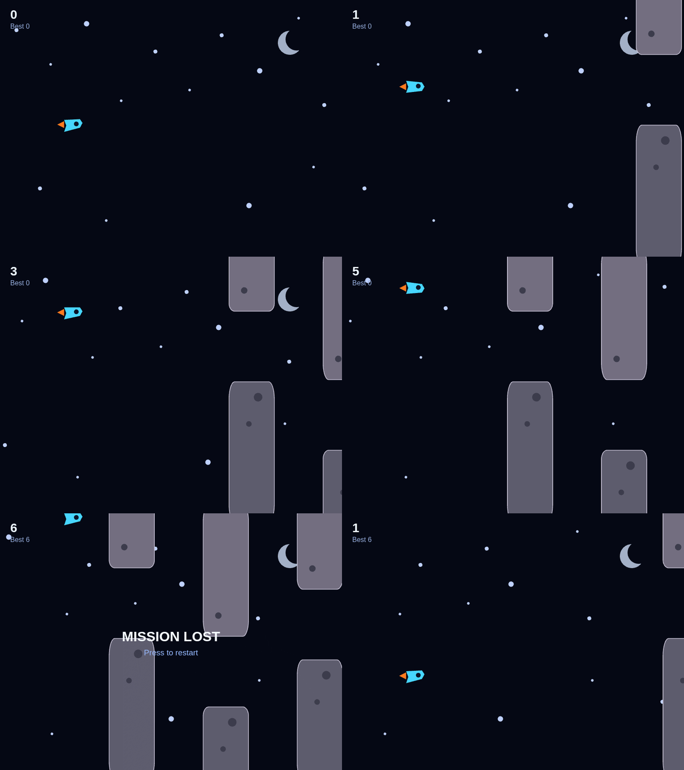
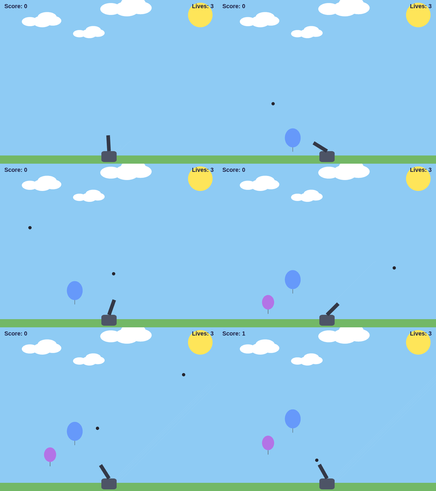

The MATLAB One-Button Game Mini Hack runs from November 2nd through November 29th, 2026! The challenge is to make a game that can be played with one button. I thought this would be a good opportunity to share some of the graphics and programming ideas behind Arcade, a collection of 15 games I developed in MATLAB using Claude Code and the MATLAB MCP Server.
Before the 2024 MATLAB Shorts Mini Hack, Tim Marston published his walkthrough of Little Nemo's airship. I learned a lot from Tim's article, and it inspired me to enter the contest. I hope that sharing some of what goes into these games might encourage a few more people to give it a try this time around as well.
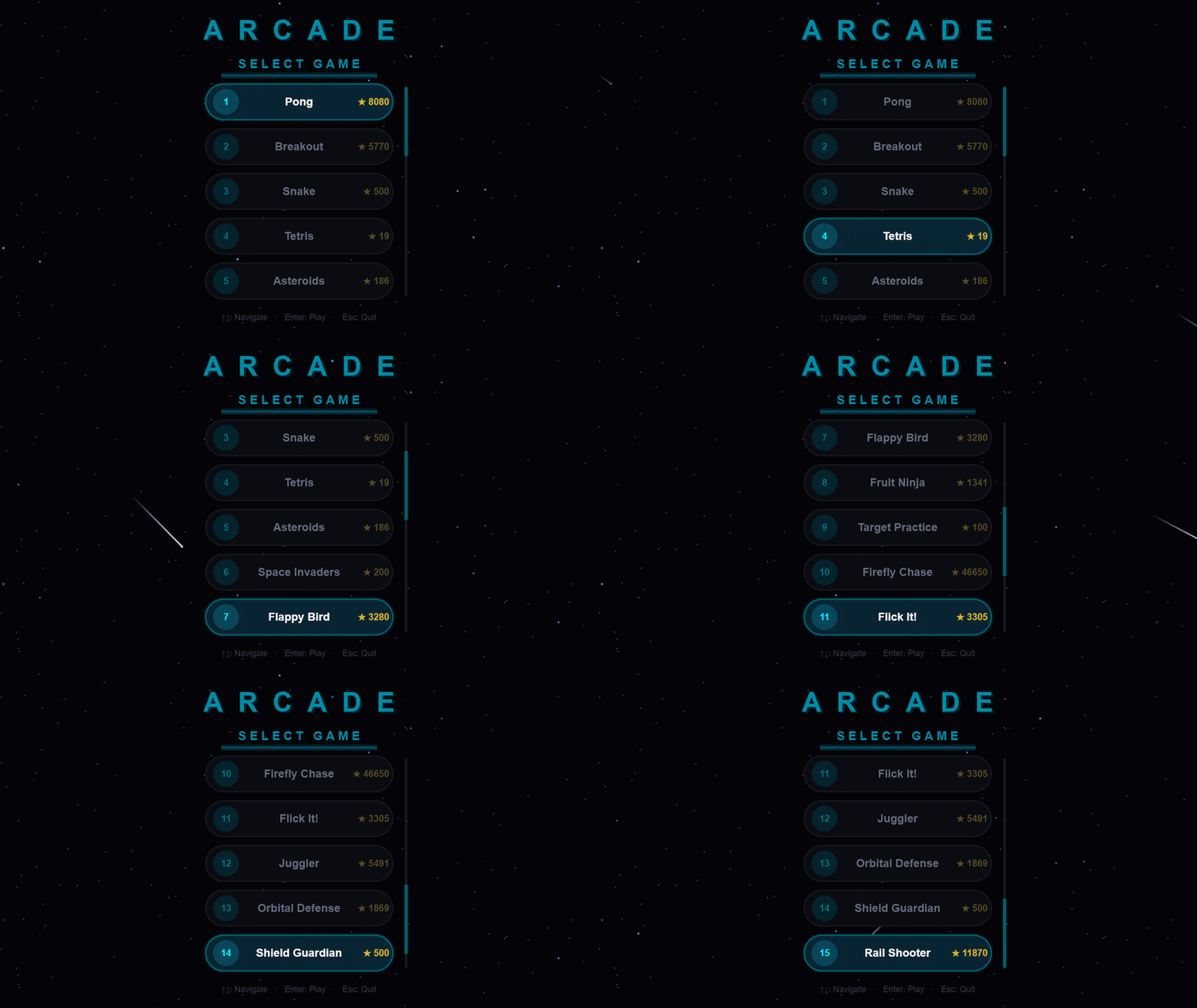
You can download Arcade from File Exchange or GitHub, add the project folder to the MATLAB search path, and run:
Arcade();
Creating and updating graphics
Arcade sports neon-styled graphics. This is accomplished by layering ordinary MATLAB graphics against a dark background. The bright colors used come from the shared GameBase palette, which enables the different games to keep a consistent appearance and accounts for quite a bit of that look.
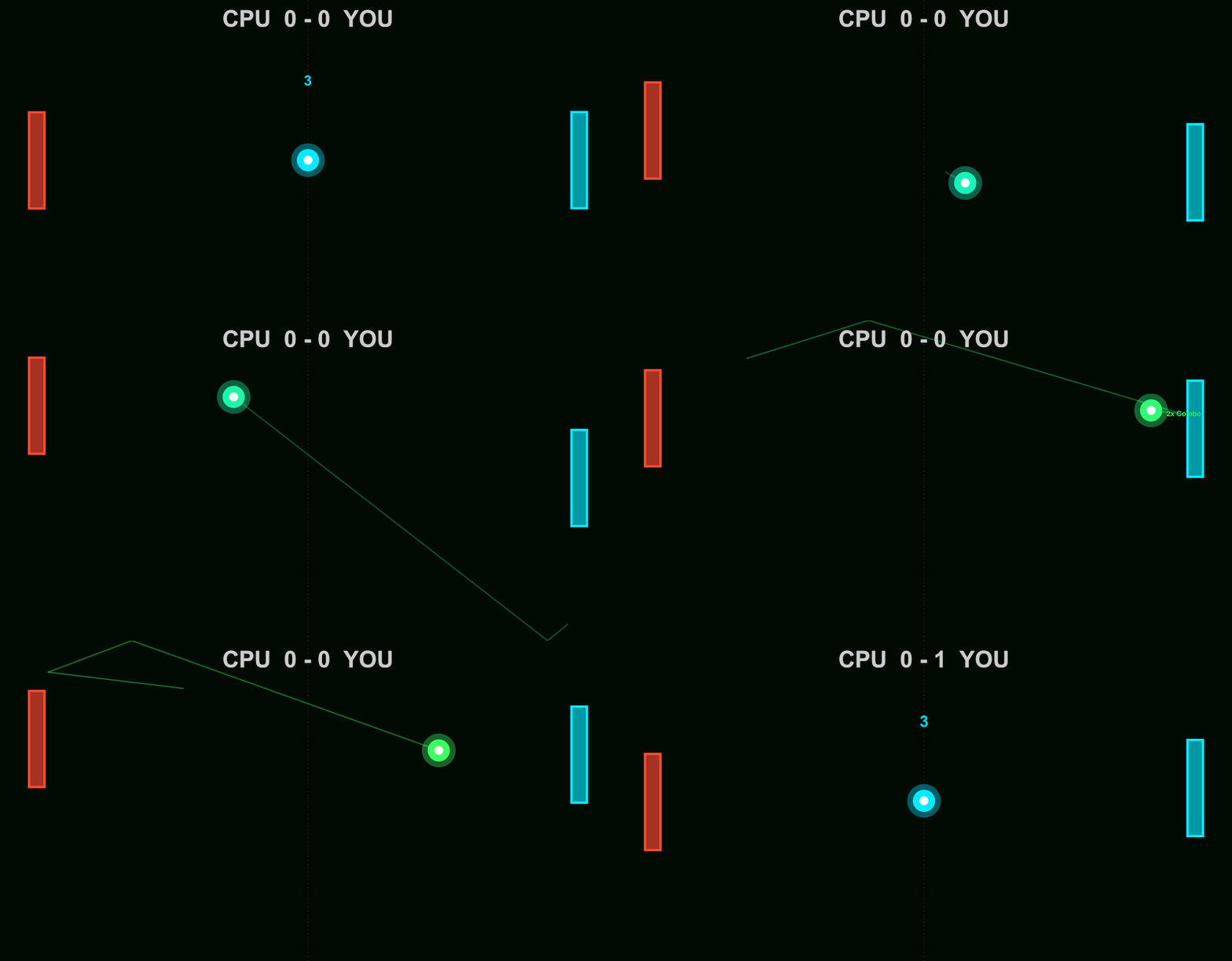
In Pong, the ball is made by drawing a colored dot, a semitransparent scatter marker and a smaller white dot at the same position. The ball and trail change from cyan through green, gold and red as the ball speeds up, while the center stays white. Against the dark background, these simple shapes give us the bright center and surrounding glow.
arcadeBallDemo();
worldSize = [854, 480];
position = worldSize / 2;
cyan = [0, 0.92, 1];
radiusParameter = max(3, round(min(worldSize) * 0.035));
baseCoreSize = 2 * radiusParameter;
baseDotSize = 5 * radiusParameter;
baseGlowArea = pi * (1.25 * radiusParameter)^2;
coloredDot = line(ax, NaN, NaN, ...
Marker=".", MarkerSize=baseDotSize, LineStyle="none", Color=[cyan, 0.15]);
glow = scatter(ax, position(1), position(2), baseGlowArea, cyan, "filled", ...
MarkerFaceAlpha=0.4);
core = line(ax, position(1), position(2), ...
Marker=".", MarkerSize=baseCoreSize, LineStyle="none", Color=[1, 1, 1, 1]);
ballLayers = {coloredDot, glow, core};
Here's how the ball looks as each layer is added:
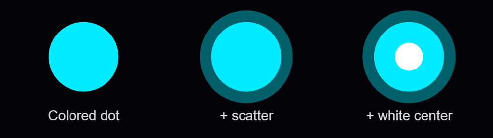
Setting NextPlot="add" preserves the existing graphics as we add the layers. Specifying the axes limits by using XLim and YLim keeps the view in place as the ball moves.
Each drawing call returns a handle to its object. With those handles stored in ballLayers, moving the ball involves assigning its new position to the existing objects:
for layerIndex = 1:numel(ballLayers)
ballLayers{layerIndex}.XData = position(1);
ballLayers{layerIndex}.YData = position(2);
end
drawnow
MathWorks' graphics-performance guidance recommends retaining graphics and updating the properties that change. Pong also checks whether its scores have changed before assigning new score text. Its trail uses preallocated position buffers, wrapping around as new positions arrive, and two retained lines display that history as a broad dim stroke with a narrower bright stroke.
Handling inputs using callback functions
The ball example responds to mouse presses through a callback function. After creating the scene, it assigns a function handle to the figure's WindowButtonDownFcn callback property:
fig.WindowButtonDownFcn = @reverseVerticalDirection;
MATLAB executes the callback function when a mouse button is pressed in the window. In the example, it is nested inside the local animateBall function:
function reverseVerticalDirection(~, ~)
velocity(2) = -velocity(2);
end
The two arguments supplied by MATLAB are the source object and event data. The ~ placeholders indicate that this function doesn't use them. As a nested function, it can access velocity in the enclosing function. Each mouse press reverses the shared vertical velocity, which the next loop iteration uses to move the ball.
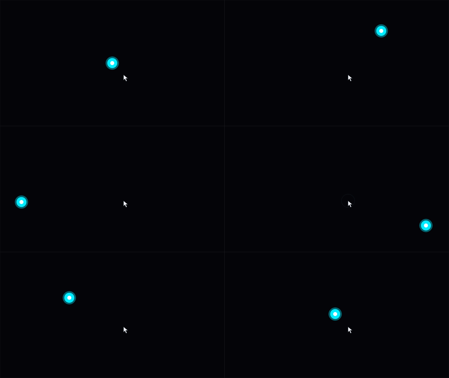
Arcade routes input through methods on the launcher. Its figure's KeyPressFcn callback property is assigned as follows, where obj is the launcher instance:
obj.Fig.KeyPressFcn = @(~, event) obj.onKeyPress(event);
The anonymous function forwards the event data to onKeyPress, where its Key property identifies the key. The launcher handles its own controls and passes appropriate input to the active game. Button release and scrolling have their own callback functions.
Mouse movement can control a paddle or aim a shot. To track the pointer as it moves within the figure, Arcade assigns a callback function to WindowButtonMotionFcn:
obj.Fig.WindowButtonMotionFcn = @(~, ~) obj.onMouseMove();
function onMouseMove(obj)
pointer = obj.Ax.CurrentPoint;
obj.MousePos = pointer(1, 1:2);
end
The axes' CurrentPoint gives the pointer position in game coordinates. MATLAB accounts for the axes' position and size, so the same code works when the playfield is resized or surrounded by margins.
On each game update, the launcher passes the stored position to the active game's onUpdate method. In Pong, obj now refers to the game instance. Once the incoming pos is available, its vertical coordinate determines the player's paddle position:
yLimits = obj.DisplayRange.Y;
if ~any(isnan(pos))
obj.PlayerPaddleY = max(yLimits(1) + obj.PaddleHalfH, ...
min(yLimits(2) - obj.PaddleHalfH, pos(2)));
end
The min and max calls keep the paddle's center at least half a paddle height from either edge. Moving the pointer into a margin therefore leaves the whole paddle inside the playfield. The graphics update then applies that position to the existing paddle patches.
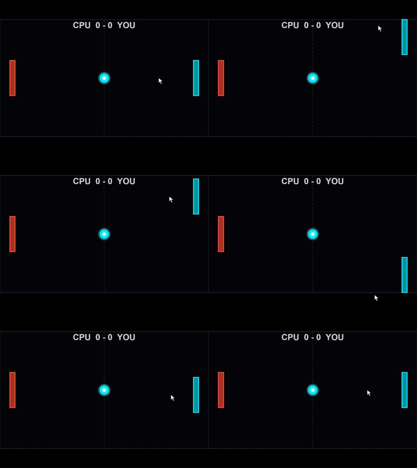
The animation loop's drawnow displays pending graphics changes and processes pending callbacks. Keeping callback functions short allows control to return to the loop promptly.
Animating visual effects
When the orb is launched in Flick It!, a call to spawnHitEffect creates a ring and rays that expand and fade. The launcher advances these shared effects alongside the active game.
In arcadeEffectsDemo.m, each click creates a burst at the mouse position, allowing several bursts to expand and fade together. To try it out, download the function, add its folder to the MATLAB path, and run:
arcadeEffectsDemo();
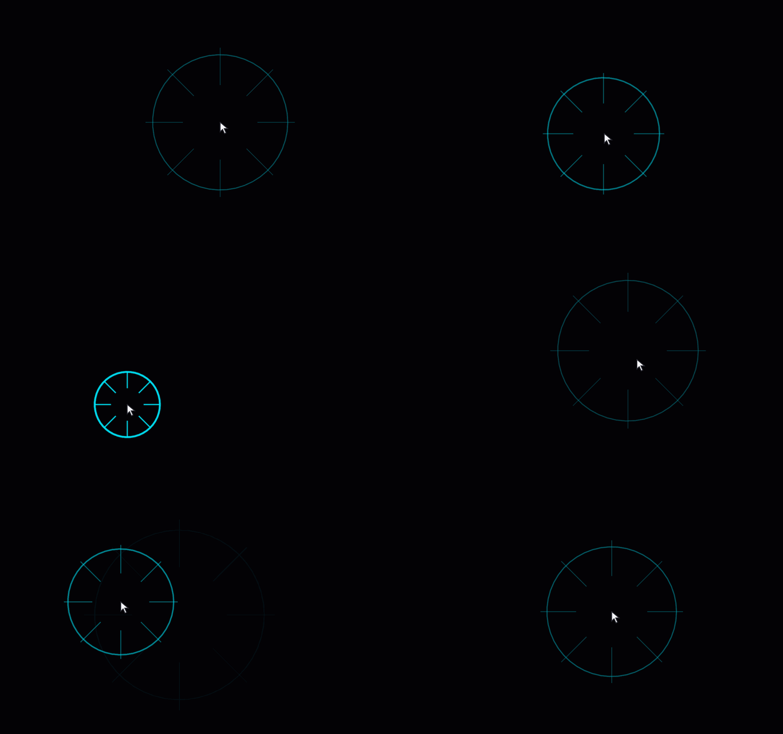
The nested callback function combines mouse-press handling with the mouse-position tracking introduced earlier. Here's the part that creates and stores a new burst:
fig.WindowButtonDownFcn = @createManualImpact;
function createManualImpact(~, ~)
point = ax.CurrentPoint;
position = point(1, 1:2);
if any(~isfinite(position)) || any(position < 0 | position > worldSize)
return
end
[newRing, newRays] = createEffect(position);
activeEffects(end+1) = struct('Ring', newRing, 'Rays', newRays, ...
'Center', position, 'AgeSeconds', 0, 'LastTime', toc(animationClock));
end
The bounds check ignores clicks outside the playfield. createEffect creates the lines, and activeEffects stores their handles, center and timing state. The animation loop updates each burst independently, allowing further clicks while earlier bursts are still expanding.
We can drive the geometry, transparency and line width from a common progress value: 0 when the burst begins and 1 at the end of its lifetime. Inside the function, the ring is updated as follows:
progress = ageSeconds / lifetimeSeconds;
eased = 1 - (1-progress)^2;
opacity = max(0, 1-1.5*eased);
ringRadius = radiusParameter * (1+2.5*eased);
ring.XData = center(1) + ringRadius*ringCos;
ring.YData = center(2) + ringRadius*ringSin;
ring.Color = [cyan, 0.8 * opacity];
ring.LineWidth = max(0.5, 3*(1-eased));
The ease-out expression starts the expansion quickly and slows it down toward the end. The burst fades out before its nominal lifetime finishes. ringCos and ringSin hold the circle's fixed directions, calculated before the loop. Arcade controls the transparency of these lines by assigning an RGBA value to Color, with alpha as the fourth component, ranging from 0 (clear) to 1 (fully opaque).
The row vectors rayCos and raySin contain the eight ray directions. Each ray joins the inner and outer radii, which increase as the burst expands:
innerRadius = radiusParameter * (0.5+1.5*eased);
outerRadius = radiusParameter * (1+3*eased);
for rayIndex = 1:numel(rays)
rays(rayIndex).XData = center(1) + [innerRadius, outerRadius]*rayCos(rayIndex);
rays(rayIndex).YData = center(2) + [innerRadius, outerRadius]*raySin(rayIndex);
rays(rayIndex).Color = [cyan, 0.6 * opacity];
rays(rayIndex).LineWidth = max(0.5, 2*(1-eased));
end
The lines are created when the burst begins, updated throughout its lifetime and deleted when it expires.
Display scaling: Keeping the scene in proportion
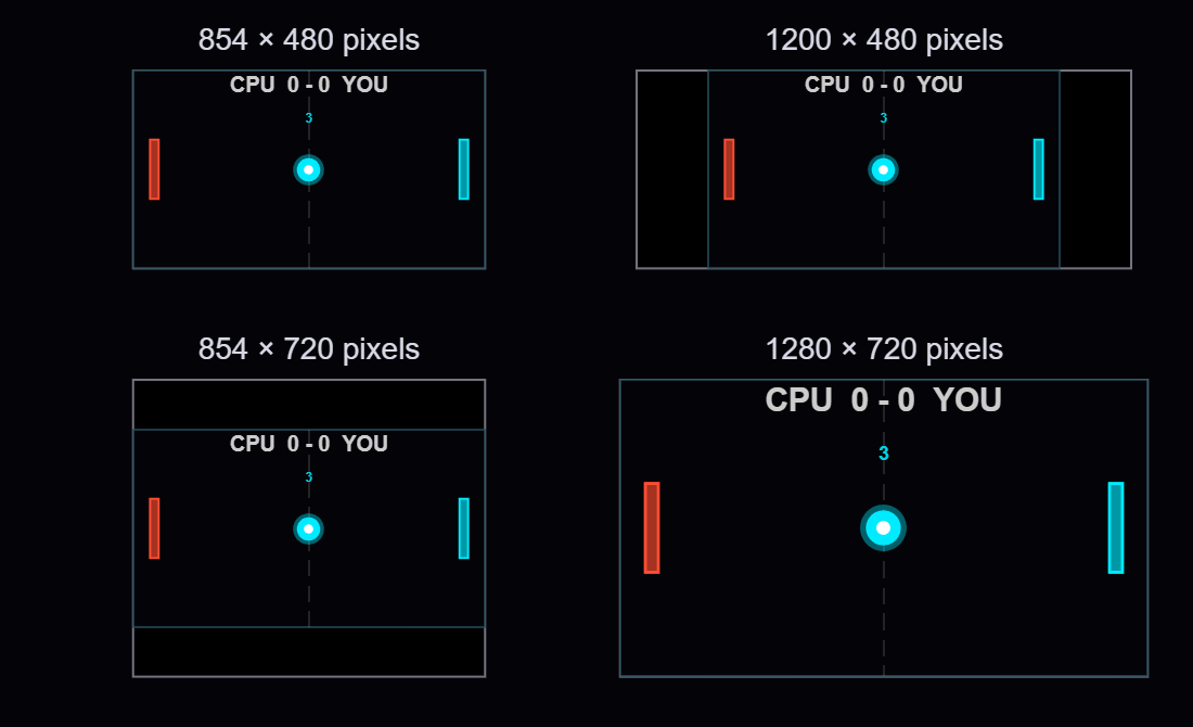
Try making the ball example's window wider while keeping its height the same. Space appears beside the playfield, and the ball still travels between the same boundaries. The example's reference window is 854 by 480 pixels, matching worldSize numerically. Resizing scales the playfield on the screen while the game's coordinate system remains unchanged.
The figure and axes use Units="pixels". Taking the min of the width and height ratios relative to the reference window gives the largest scale factor that fits in both directions. Applying that same scale to both dimensions preserves the playfield's 16:9 aspect ratio.
For a 1200-by-480 window, the height limits the scale to 1. The fitted area remains 854 by 480, leaving (1200-854)/2 = 173 pixels on each side. In a 1280-by-720 window, the playfield grows to approximately 1.5 times its reference width and height. Here are four window sizes at a common page scale:
MATLAB already scales graphics defined in data coordinates as the axes resize. For example, a paddle drawn with patch grows with the axes. In the example, marker sizes, font sizes and line widths use points, while scatter sizes use points squared.

To make a circle twice as wide, we need four times its area. Doubling SizeData multiplies its width by only √2:
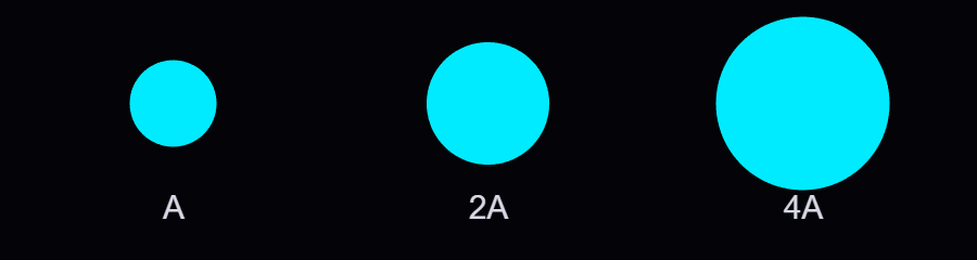
fig.SizeChangedFcn = @fitScene;
The nested fitScene callback function combines the axes calculation with these size updates:
function fitScene(~, ~)
if ~isgraphics(ax)
return
end
availableSize = max(fig.Position(3:4), [1, 1]);
displayScale = min(availableSize ./ worldSize);
fittedSize = worldSize * displayScale;
ax.Position = [(availableSize - fittedSize)/2 + 1, fittedSize];
% Always derive sizes from their reference values
core.MarkerSize = baseCoreSize * displayScale;
coloredDot.MarkerSize = baseDotSize * displayScale;
glow.SizeData = baseGlowArea * displayScale^2;
instruction.FontSize = baseFontSize * displayScale;
playfield.LineWidth = 0.5 * displayScale;
end
The first two entries of ax.Position set the left and bottom position, splitting the unused space equally between opposite sides. The last two give the fitted width and height. The axes limits remain unchanged, so movement and collision calculations keep using the same game coordinates.
At scale 1.5, the marker sizes are multiplied by 1.5 and the scatter area by 2.25. The updated sizes are calculated from their stored reference values. A 34-point reference marker becomes 51 points at scale 1.5, then 68 points at scale 2.
You can also use Units="normalized" to size and position the axes relative to the figure. Arcade's axes setup uses [0 0 1 1] to allocate the full available area:
obj.Ax = axes(obj.Fig, "Units", "normalized", "Position", [0 0 1 1]);
obj.Ax.XLim = obj.DisplayRange.X;
obj.Ax.YLim = obj.DisplayRange.Y;
Arcade's resize method obtains the available dimensions in pixels with getpixelposition and calculates the same display scale. It uses pbaspect to preserve the playfield's aspect ratio. MATLAB fits the playfield within the available space, leaving margins where needed:
axPx = getpixelposition(obj.Ax);
newPs = min(axPx(3) / 854, axPx(4) / 480);
gameAR = diff(obj.DisplayRange.X) / diff(obj.DisplayRange.Y);
pbaspect(obj.Ax, [gameAR 1 1]);
For Arcade, I also wanted markers, text and line widths to grow proportionally with the playfield. MATLAB also supports automatic resizing for text through FontUnits="normalized", which expresses font size as a fraction of the axes plot box height. This works well for text in a playfield with a fixed aspect ratio. Arcade's shared resize helper modifies current property values, using the ratio of the new scale to the previous scale; for example, moving from 51 to 68 points requires multiplying by 2/1.5. The function applies a common display scale to text, markers and line widths, in order to preserve their relative sizes as the window is resized.
FPS scaling: Let elapsed time determine the motion
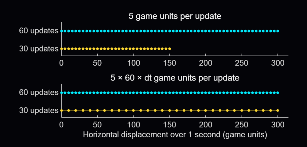
Suppose that the ball moves 5 game units on each update. At 60 updates per second it travels 300 units in a second, but at 30 it travels only 150. Calculating the state, drawing and processing input all contribute to the time between updates, so we need to measure that interval to maintain a consistent speed.
Gianluca Carnielli discusses the relationship between time and animation frames in Animating Science: Creating Time-Sensitive Animations with MATLAB. In his example, he explains how to create a frame-based animation from time-based coordinates, by choosing the video’s duration and frame rate, calculating the simulation timestep between two consecutive frames, and resampling the coordinates using retime.
In a live game, we process player actions and calculate each new state using the time elapsed since the previous update. Arcade expresses many motion parameters per reference interval, using 60 frames per second (FPS) as its reference frequency. An elapsed time of 1/60 seconds represents 1 reference interval, while 1/30 seconds represents 2. In the example, we define the velocity and reference frequency before the loop and start the clock with tic once the initial scene is displayed:
velocity = [5, 3]; % Game units per reference interval
referenceFPS = 60; % Reference intervals per second
animationClock = tic;
previousTime = 0;
currentTime = toc(animationClock);
dtSeconds = min(currentTime - previousTime, 0.1);
previousTime = currentTime;
dtScale = dtSeconds * referenceFPS;
position = position + velocity * dtScale;
Here dtSeconds is in seconds, and dtScale counts reference intervals. A horizontal velocity of 5 now gives a movement of 10 game units over 1/30 second. Taking 30 steps of 10 units covers the same 300 units as 60 steps of 5 units. The samples are farther apart, so the motion can look less smooth:
The min(..., 0.1) caps a single represented interval at 0.1 seconds (10 FPS) to limit jumps after a stall. If an update arrives after 0.5 seconds, the code advances only 0.1 seconds, and the remaining 0.4 seconds are discarded.
The reference frequency is 60 FPS; the actual update rate depends on execution. We could also use game units per second and write position = position + velocityPerSecond * dtSeconds.
Arcade schedules its updates with a timer. The callback function assigned to its TimerFcn property calls the launcher's frame-update method:
obj.RenderTimer = timer(ExecutionMode="fixedSpacing", ...
Period=0.02, TimerFcn=@(~, ~) obj.onFrame());
start(obj.RenderTimer)
With fixedSpacing, the period begins after the preceding callback function finishes. The function's own work therefore contributes to the interval between updates. The launcher measures the full interval and passes the resulting time scale to the active game.
arcadeBallDemo(Inf, 0.04);
Its measured interval includes both the pause and the surrounding work. Both Arcade and the example use the full drawnow command. The limitrate option can reduce rendering work by limiting display updates to 20 per second; its suitability depends on the animation's required display rate.
Flick It! multiplies its velocity by friction^dtScale, where friction is the fraction of velocity retained over one reference interval. Over 2 intervals, the multiplier is the square of that factor, equivalent to applying it once in each interval. This makes the velocity decay follow the elapsed time.
For accelerating objects, the numerical approximation can still change with step size, and collisions need to account for movement between samples. Pong checks when the ball crosses the paddle's front face and interpolates its vertical position there, allowing a contact to be detected between two displayed positions.
Organizing games using classes
Arcade's registry stores a constructor function handle for each game. When a game is selected, the launcher calls the corresponding constructor to instantiate the game class. Here's an adaptation of the launch sequence, with Pong selected explicitly and obj referring to the launcher:
createGame = @games.Pong;
game = createGame();
game.FontScale = obj.FontScale;
game.init(obj.Ax, obj.DisplayRange)
game.beginGame()
obj.ActiveGame = game;
Each game subclasses engine.GameBase. The shared init method sets up the session and calls the game's onInit, which creates its state and graphics. Assigning FontScale beforehand lets newly created markers and text use the current display size. The launcher stops its render timer before creating the game and restarts it after the initialized game is assigned to ActiveGame. This prevents timer callbacks from running while the game’s state and graphics are being created.
GameBase declares four abstract methods that each game class must implement:
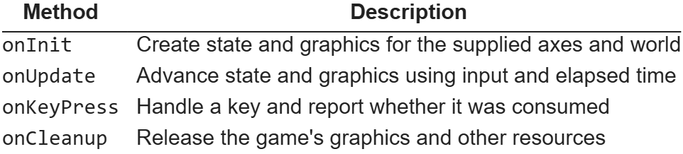
The launcher calls onUpdate on its active game, and MATLAB dispatches that call to the selected subclass. Pong implements paddle and ball movement; Flappy Bird advances its bird and pipes. All games inherit methods for scoring, combo handling and visual effects from GameBase. Window management, menus, timing and common services stay with the launcher.
As a handle class, GameBase lets the launcher keep a reference to the same game instance while its state changes. Position arrays, velocities, scores and graphics handles belong to that instance. Property access attributes allow the host to read the common score while leaving changes under the control of the game classes.
Flappy Bird creates its pipe patches in onInit, then reuses them throughout the game. Their handles and state are stored in private properties of the game instance. Its onUpdate method moves the active pipes across the playfield. Spawning a pipe selects an available pair, assigns its position and gap, and adds it to the active list. Once it leaves the playfield, the pair is hidden and its slot becomes available again:

In the default gravity-and-flap mode, the onKeyPress input handler sets a pending flap flag. The next update applies the upward impulse and clears the flag.
When the window closes, Arcade stops and deletes its timer, calls the active game's onCleanup method and clears its effects before deleting the figure. The smaller examples use MATLAB's onCleanup object to delete their own figure when the function exits. The requestClose callback function assigned to the figure’s CloseRequestFcn property sets a stop flag, letting the current update finish before cleanup removes the graphics.
Recent work on MATLAB graphics and performance
The MathWorks graphics team has also been improving the underlying rendering system. Maddie Moon's article about WebGL describes the R2025a transition, which brought the renderer already used by uifigure to regular MATLAB figures, along with work on stability, consistency and smoothing. Will Jackson also explains related changes to built-in panning, zooming and rotation in his article on the new interactions system.
R2025b focused on quality and stability improvements, building on the changes introduced in R2025a. It also improved performance when capturing successive frames in a loop with getframe, the function used by Arcade’s recording helper to capture and store frames for GIFs and videos.
R2026a included memory and stability improvements for graphics such as scatter and surface plots, described in Adam Danz's overview and the release notes. In addition, Jessa Karlberg describes the redesigned axes toolbar in R2026a, which allows seamless hovering without the animation slowdown issues caused by the toolbar’s continuous mouse tracking in earlier releases, eliminating the need to remove the toolbar as a workaround.
R2026b improved responsiveness for large data visualizations, with plot and plot3 being able to display lines and markers incrementally and shortening the wait time for the first visible results. MathWorks also reports automatic selection of a dedicated rendering GPU on supported Windows and Linux systems with multiple GPUs. These changes are documented in the release notes and the GPU-selection update.
info = rendererinfo;
info.GraphicsRenderer
info.RendererDevice
Mike Croucher also describes a new object-management system for R2026b, which can speed up object-oriented MATLAB code by reducing the cost of creating and deleting objects, as well as accessing their properties. The system is currently available as a beta and can be enabled through a package on File Exchange. Its documentation explains the changes to object lifecycle and compatibility.
Developing MATLAB code with AI
Arcade was developed with Claude Code through the MATLAB MCP Server, and the contest welcomes AI assistance as an option.
When working with an AI assistant, consider sharing your project's requirements and any existing code it can build on. Arcade's developer guide, for example, describes the shared game interface and explains how to add a new game. For your own game, you could begin with the main interaction and add features gradually, playing and improving it as you go. When something goes wrong, describe what happened and how to reproduce the problem, such as a ball passing through a wall at higher speeds.
The MATLAB Agentic Toolkit provides workflows for code review, analysis and testing. Its setup guide covers connecting MATLAB to AI applications including Claude Code, GitHub Copilot, OpenAI Codex, Gemini CLI and Amp, and installing MATLAB-specific skills. Through the MCP server, the AI assistant can run MATLAB code and tests, inspect the results, and use them to help diagnose problems and revise the code.
Several implementation choices in Arcade align with the MATLAB Coding Guidelines and performance rules: using a handle class for an object whose identity persists, restricting access to its state, retaining graphics, preallocating known-size arrays and cleaning up timers. The two downloadable examples presented above were checked with MATLAB Code Analyzer and tested for resizing, input, handle reuse and cleanup.
I hope that this article gives you something to experiment with, and perhaps a starting point for the One-Button Game Mini Hack. I look forward to seeing what you make!

Hi there,
Is there a change in the json response when I do http write to a channel ?
I send:
POST /update.json HTTP/1.1
Content-Type: application/x-www-form-urlencoded
Host: api.thingspeak.com
Connection: close
Content-Length: 102
apikey=xxxxxxxxxxxx&field1=-4.803&field3=18&field4=91&field5=109&field6=56&field7=0&field8=7
and I don't receive the normal response
I get sth like:
'unsafe-eval'; style-src 'self' https: 'unsafe-inline'; connect-src 'self' https: https://*.mathworks.com https://*.thingspeak.com https://*.omtrdc.net https://*.demdex.net; frame-src 'self' https: https://*.mathworks.com
I built Beat the PID for the One-Button Game Mini Hack: Beat the PID. Each tap switches an actuator on or off, and you try to hold a trace inside a moving band across six plants, from a thermostat to an inverted pendulum. A PID ghost plays the same level with the same on/off limit.
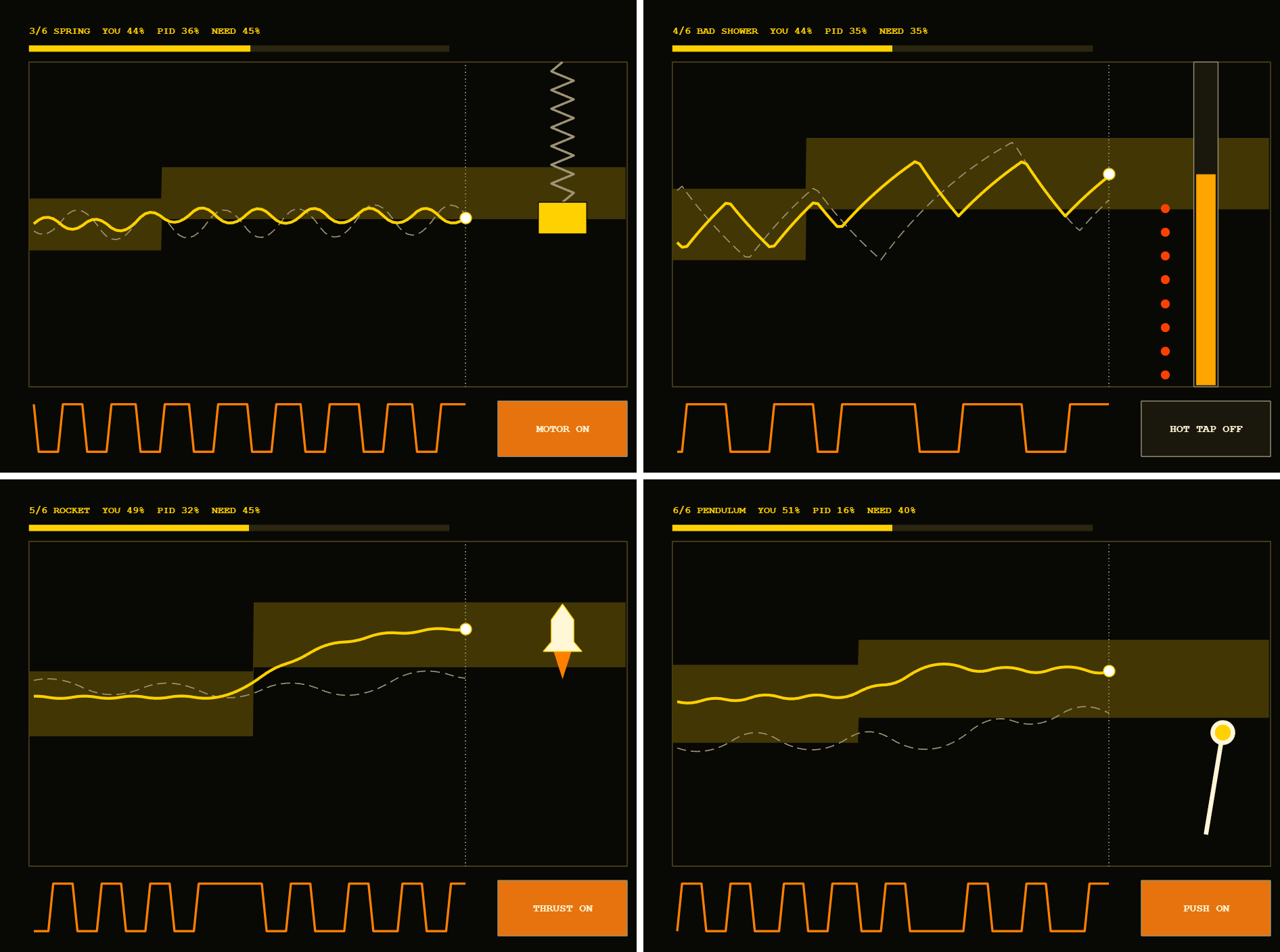
The yellow line is you, and the dashed gray line is the PID ghost. The band scrolls in from the right so you can plan ahead.
These are the things that surprised me, with measurements where I have them. I built it with help from an AI coding assistant (Claude Code), and we tested each change in MATLAB.
1. The character limit counts reformatted code
My first local count, with comment lines removed, said 9,862 characters. minihackContest.validate said 12,253. The validator's number matched this exactly:
code = char(tree2str(mtree(fileread('game.m'))));
numel(code)
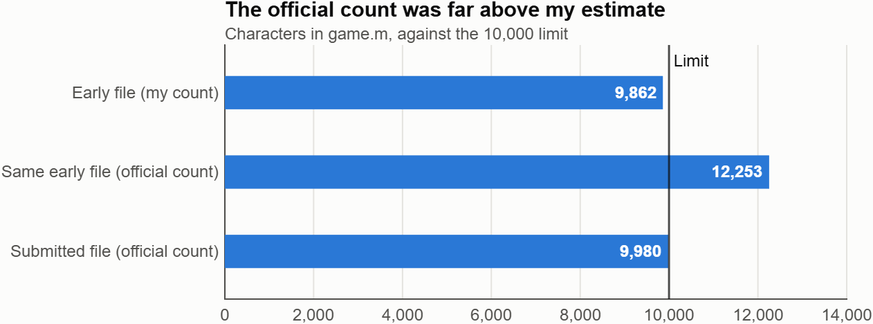
mtree and tree2str are undocumented, so treat this as a useful local estimate. It matched on my game at several sizes and on another contest entry.
Reformatting changes what costs characters:
% What you write
ax.Color=[.035 .045 .07];
% What gets counted
ax.Color = [ .035, .045, .07 ];
- Comments are free, so comment generously.
- Squeezing out spaces saves nothing, because they get added back.
- Every value in an array costs extra for its comma and spacing.
- Each nesting level costs 4 characters per line. Moving a deep block into its own function can pay for itself.
- Grouping assignments helps:
[s.t,s.acc,s.in,s.ing,s.ei,s.dwg,s.n] = deal(0);
Those changes, along with cutting a few visual extras, took my game from 12,253 to under 10,000 and kept all six levels.2. min and max ignore NaN
I used NaN for trace samples not recorded yet, then clamped values to the scope:
max(-.02,min(1.02,NaN)) % returns 1.02, not NaN
Because min and max ignore NaN, every empty sample became a real value at the top of the scope and drew a stray line. If you need clamping, restore the gaps afterward with y(isnan(v)) = nan.3. Use a fixed physics step and expm
dt varies between frames, so I run the physics at a fixed 120 Hz and spend the elapsed time in whole steps:
s.acc = s.acc+dt;
while s.acc >= s.h && s.t < s.T && ~s.crash
s.acc = s.acc-s.h;
s = stepPlant(s);
end
Each plant is linear, x' = Ax + B[u;1], so I can discretize it exactly once at startup:
n = size(A,1);
M = expm([A B;zeros(2,n+2)]*h);
Ad = M(1:n,1:n);
Bd = M(1:n,n+1:n+2);
Each physics step is then just x = Ad*x + Bd*[u;1]. The contest player limits dt to 0.05 s, so a game running under 20 fps plays in slow motion, but the physics stays stable and each step stays the same.4. A one-button PID is a relay
The ghost's PID output doesn't set a power level. Its sign picks on or off, and a minimum switching interval stops it from toggling faster than a person could:
e = r-y;
ei = max(-.3,min(.3,ei+e*h));
v = e+Ki*ei-Kd*(y-yPrev)/h;
if timeSinceSwitch >= minDwell && (v > 0) ~= u
u = v > 0;
timeSinceSwitch = 0;
end
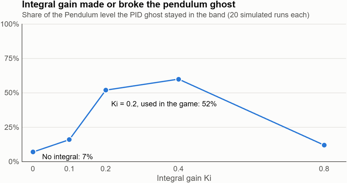
The integral term matters more than I expected on a relay. On the inverted pendulum level, the ghost averaged 52% of the time in the band with Ki = 0.2, and 7% with Ki = 0. These are averages from simulated runs at one set of gains, and the result is very sensitive to tuning.
5. Measure work and frame rate separately
MATLAB Online was by far the biggest performance surprise. On my connection, the same game behaved very differently:
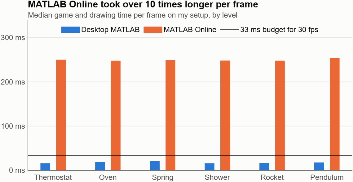
Median game and drawing time per frame. I measured MATLAB Online on a slightly earlier build, before the final color and text changes.
The MATLAB Online time was almost the same on all six levels, even though each draws different things, so I suspect a fixed delay and not my drawing load. Other games lagged for me there too. Your results may differ, so test your own game there.
Two habits helped:
- Time the work, not just the frame. On my Windows PC, a paced loop took about 46 ms per frame even when the actual work was about 10 ms, because pause overshot. Frame rate alone would have sent me after the wrong problem.
- Send only what changed. Create graphics once, set fixed X data once, and update only Y data. My render also skips frames where nothing changed, which keeps idle menus quiet and still gives the same result if called twice:
st = [s.mode s.lv s.t s.u];
if isequal(s.ax.UserData,st)
return
end
s.ax.UserData = st;
A piecewise-constant band needs vertices only at its ends and steps, which cut it from up to 166 numbers per update to a handful. Scrolling the scope at 15 Hz while moving the player marker every frame also reduced updates without making the controls feel slower.Play it on the desktop
If the game crawls in MATLAB Online, you can run it in desktop MATLAB:
- Download the starter project, unzip it, and open minihackContest.prj. Opening the project installs the contest tools.
- Copy my entry's code into the project's game.m.
- Run minihackContest.play.
Tap Space or click to play. I'd love to know which plant beats you, and whether anyone can beat the PID on all six.

Hello everyone, I hope you all had a fantastic MATLAB EXPO! I wanted to create a forum for people to ask follow-up questions or start discussions related to the workshop Hands-On Agentic AI for Engineered Systems with MATLAB and Simulink. We ran this workshop nine (!) times over the two days of MATLAB EXPO, and heard some incredibly insightful comments and questions in each session, so I wanted to make a central bulletin board for people to share their thoughts and hear insights. A few ideas:
- What did you most enjoy about the workshop?
- Are there any topics/exercises that weren't clear, or maybe an area you want to explore more?
- Do you have an idea for how you'd like to apply agentic AI in your work?
MATLAB EXPO may be over, but that doesn't mean the conversation has to end!

This Week's Quiz
157 responses

By SunHuilin
What happens when a tiny pixel cat tries on eight different personalities? Sometimes you get instant cuddles. Sometimes your sofa gets a new ruler.
Purrfect Fit is my entry for the MATLAB One-button Game Mini Hack. Different pairs of eyes scroll through a cat's glasses. Tap or press SPACE to stop them. Fit the eyes inside the frames, and the kitty reveals its personality with a short message and matching pixel effects. Miss the target, and the kitty offers a little encouragement. Tap again to try another round.
Play the game: Purrfect Fit
Here are four techniques behind the game. The snippets below are simplified illustrations of the implementation, rather than a complete runnable game.

1. Treat an RGB array as a tiny canvas
The artwork starts as a 150-by-200-by-3 RGB array, displayed across an 800-by-600 game area. One artwork pixel occupies four game-coordinate units in each direction. Rectangles, filled polygons, and small bitmap patterns build the cat, glasses, lettering, and effects without loading external image files.
The key is to create the image object once, then update its CData:
% During initialization:
h = image(ax,[2 798],[2 598],background);
% During rendering:
frame = background;
% Draw the moving elements into frame here.
h.CData = frame;
The static background is prepared during initialization. Each render starts with that background and adds the animated elements. This avoids accumulating drawing operations from previous frames and keeps the number of graphics objects fixed.
I also draw the title with small bitmap letters. That gives the main heading a consistent pixel style without depending on an installed pixel font. The longer instructions and feedback use MATLAB text objects for readability.
2. Separate scrolling, stopping, and feedback
The game has three states: scrolling, success, and miss. The same button stops the eyes during scrolling and starts another round after the result.
Scrolling uses elapsed time rather than a fixed distance per update:
phase = mod(phase + speed*dt,192);
There are eight eye designs, each occupying a 24-row tile, so the strip repeats after 192 artwork pixels. Using dt makes the intended scrolling speed independent of the number of updates per second, although a slow display can still make fast motion harder to judge.
One small detail matters: when a press arrives, I check the current phase before advancing the strip. This keeps the timing decision tied to the state that was just rendered.
The fit test uses the visible vertical bounds of each eye design. Both bounds must lie inside the target opening; checking only the center could accept eyes that still stick out of the frame. On success, the strip snaps to the centered position for the final portrait.
A brief restart guard prevents an immediate second press from dismissing the result before the player can read it.
3. Animate the tail with a small coordinate shift
The cat's tail uses filled polygons. Instead of storing multiple animation frames, I shift their horizontal coordinates with a sine wave:
d = 3*sin(t*3);
x = x + round(d*(118-y)/21);
The vertical weighting keeps the base relatively steady while the tip moves more. Rounding preserves the pixel-art appearance.
Layering is just as important as motion. I draw the moving tail first, restore the static foreground artwork through a mask, and then draw the eyes and glasses. This keeps the tail behind the body and prevents it from painting over the face.
4. Store small patterns compactly, then reuse them
The eight eye styles share a palette and a common rendering path. Their pixel data is stored as compact runs and decoded during initialization, so rendering can reuse the prepared arrays.
The personality effects use a different representation: seven integers describe a 7-by-7 binary pattern. Each bit says whether one pixel is filled:
if bitget(pattern(row),8-col)
% Draw this pixel using the personality's color.
end
The same drawing loop produces paws, lightning bolts, sleepy Zs, sparkles, spirals, question marks, hearts, and musical notes. Changing the pattern and color gives each personality its own visual feedback without duplicating the effect renderer.
The messages work similarly: each eye style has three possible success lines, while misses draw from a shared pool of encouraging phrases. For example:
- Fierce: "Tiny paws. Big boss energy."
- Sleepy: "Wake me when snacks arrive."
- Loving: "Can I keep you, human?"
- Miss: "Oops! Let's blame the whiskers."
Random choices happen when a round starts or a result is selected. Rendering reads those choices, so the message does not change every frame.
What helped most under the character limit
The biggest savings came from reusing drawing routines, palettes, and animation logic, and from compact representations of the artwork. Shorter variable names helped too, but shared structure saved more space than shortening names alone.
The current build passed the official validator at 8,933 counted code characters. During compression, I compared rendered frames and seeded update sequences with the previous version to check that the smaller code preserved the existing appearance and gameplay.
My favorite part is that the eyes change more than the cat's expression: they change the little conversation you have with it.
Which personality would you add next: a suspicious detective kitty, a dramatic movie-star kitty, or something even stranger?
Development note: I used OpenAI Codex to assist with coding, iteration, and code review.
When the agent tunes the controller, what stops it from passing the specs on the nominal model but failing on delay, saturation, or parameter variation? Do you make it run a robustness sweep, not just one simulation?
Hello MATLAB EXPO community! Now that everybody has had a chance to digest all of the exciting sessions you saw last week, I wanted to create a forum for further discussion of @Emmanouil Tzorakoleftherakis and I's session, Building Embedded Controllers with Agentic AI and Model-Based Design. Do you have questions, comments, or feedback following the session? Let us know! Some points to consider for discussion:
- What was something interesting you learned from the session?
- What is something you'd like to learn more about after having watched the session?
- How comfortable are you with the prospect of AI agents designing controllers? Did the session change that feeling at all?
We'd love to see your thoughts below!

Hello everyone. I am noob at coding and want to learn advance level of matlab and i want a book for me to help me learn from scratch and make sure its well thing and i am mostly interested in mechatronics like how a system acts and behaves so please give me some reccomandation also i am frustated.
Informazioni su Discussions
Discussions is a user-focused forum for the conversations that happen outside of any particular product or project.
Get to know your peers while sharing all the tricks you've learned, ideas you've had, or even your latest vacation photos. Discussions is where MATLAB users connect!
Get to know your peers while sharing all the tricks you've learned, ideas you've had, or even your latest vacation photos. Discussions is where MATLAB users connect!
Altre aree comunitarie

MATLAB Answers
Poni e rispondi a domande su MATLAB e Simulink

Scambio di file
Scarica o contribuisci al codice inviato da un utente

Cody
Risolvi problemi, impara ad usare MATLAB e ottieni badge

Blog
Scopri MATLAB e Simulink dall’interno

Area giochi di chat AI
Utilizza l'intelligenza artificiale per generare la bozza iniziale del codice MATLAB e rispondere alle domande!

