eqn =
Risultati per
The int function in the Symbolic Toolbox has a hold/release functionality wherein the expression can be held to delay evaluation
syms x I
eqn = I == int(x,x,'Hold',true)
which allows one to show the integral, and then use release to show the result
release(eqn)
Maybe it would be nice to be able to hold/release any symbolic expression to delay the engine from doing evaluations/simplifications that it typically does. For example:
x*(x+1)/x, sin(sym(pi)/3)

If I'm trying to show a sequence of steps to develop a result, maybe I want to explicitly keep the x/x in the first case and then say "now the x in the numerator and denominator cancel and the result is ..." followed by the release command to get the final result.
Perhaps held expressions could even be nested to show a sequence of results upon subsequent releases.
Held expressions might be subject to other limitations, like maybe they can't be fplotted.
Seems like such a capability might not be useful for problem solving, but might be useful for exposition, instruction, etc.
I am very excited to share my new book "Data-driven method for dynamic systems" available through SIAM publishing: https://epubs.siam.org/doi/10.1137/1.9781611978162
This book brings together modern computational tools to provide an accurate understanding of dynamic data. The techniques build on pencil-and-paper mathematical techniques that go back decades and sometimes even centuries. The result is an introduction to state-of-the-art methods that complement, rather than replace, traditional analysis of time-dependent systems. One can find methods in this book that are not found in other books, as well as methods developed exclusively for the book itself. I also provide an example-driven exploration that is (hopefully) appealing to graduate students and researchers who are new to the subject.
Each and every example for the book can be reproduced using the code at this repo: https://github.com/jbramburger/DataDrivenDynSyst
Hope you like it!
It would be nice to have a function to shade between two curves. This is a common question asked on Answers and there are some File Exchange entries on it but it's such a common thing to want to do I think there should be a built in function for it. I'm thinking of something like
plotsWithShading(x1, y1, 'r-', x2, y2, 'b-', 'ShadingColor', [.7, .5, .3], 'Opacity', 0.5);
So we can specify the coordinates of the two curves, and the shading color to be used, and its opacity, and it would shade the region between the two curves where the x ranges overlap. Other options should also be accepted, like line with, line style, markers or not, etc. Perhaps all those options could be put into a structure as fields, like
plotsWithShading(x1, y1, options1, x2, y2, options2, 'ShadingColor', [.7, .5, .3], 'Opacity', 0.5);
the shading options could also (optionally) be a structure. I know it can be done with a series of other functions like patch or fill, but it's kind of tricky and not obvious as we can see from the number of questions about how to do it.
Does anyone else think this would be a convenient function to add?
My favorite image processing book is The Image Processing Handbook by John Russ. It shows a wide variety of examples of algorithms from a wide variety of image sources and techniques. It's light on math so it's easy to read. You can find both hardcover and eBooks on Amazon.com Image Processing Handbook
There is also a Book by Steve Eddins, former leader of the image processing team at Mathworks. Has MATLAB code with it. Digital Image Processing Using MATLAB
You might also want to look at the free online book http://szeliski.org/Book/
In the past two years, large language models have brought us significant changes, leading to the emergence of programming tools such as GitHub Copilot, Tabnine, Kite, CodeGPT, Replit, Cursor, and many others. Most of these tools support code writing by providing auto-completion, prompts, and suggestions, and they can be easily integrated with various IDEs.
As far as I know, aside from the MATLAB-VSCode/MatGPT plugin, MATLAB lacks such AI assistant plugins for its native MATLAB-Desktop, although it can leverage other third-party plugins for intelligent programming assistance. There is hope for a native tool of this kind to be built-in.
Hello! The MathWorks Book Program is thrilled to welcome you to our discussion channel dedicated to books on MATLAB and Simulink. Here, you can:
- Promote Your Books: Are you an author of a book on MATLAB or Simulink? Feel free to share your work with our community. We’re eager to learn about your insights and contributions to the field.
- Request Recommendations: Looking for a book on a specific topic? Whether you're diving into advanced simulations or just starting with MATLAB, our community is here to help you find the perfect read.
- Ask Questions: Curious about the MathWorks Book Program, or need guidance on finding resources? Post your questions and let our knowledgeable community assist you.
We’re excited to see the discussions and exchanges that will unfold here. Whether you're an expert or beginner, there's a place for you in our community. Let's embark on this journey together!
初カキコ…ども… 俺みたいな中年で深夜にMATLAB見てる腐れ野郎、 他に、いますかっていねーか、はは
今日のSNSの会話 あの流行りの曲かっこいい とか あの 服ほしい とか ま、それが普通ですわな
かたや俺は電子の砂漠でfor文無くして、呟くんすわ
it'a true wolrd.狂ってる?それ、誉め 言葉ね。
好きなtoolbox Signal Processing Toolbox
尊敬する人間 Answersの海外ニキ(学校の課題質問はNO)
なんつってる間に4時っすよ(笑) あ~あ、休日の辛いとこね、これ
-----------
ディスカッションに記事を書いたら謎の力によって消えたっぽいので、性懲りもなくだらだら書いていこうと思います。前書いた内容忘れたからテキトーに書きます。
救いたいんですよ、Centralを(倒置法)
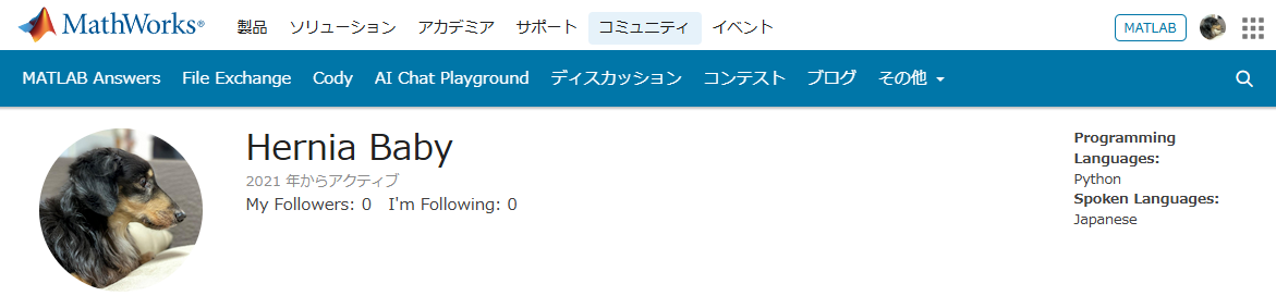
いっぬはMATLAB Answersに育てられてキャリアを積んできたんですよ。暇な時間を見つけてはAnswersで回答して承認欲求を満たしてきたんです。わかんない質問に対しては別の人が回答したのを学び、応用してバッジもらったりしちゃったりしてね。
そんな思い出の大事な1ピースを担うMATLAB Centralが、いま、苦境に立たされている。僕はMATLAB Centralを救いたい。
最悪、救うことが出来なくともCentralと一緒に死にたい。Centralがコミュニティを閉じるのに合わせて、僕の人生の幕も閉じたい。MATLABメンヘラと呼ばれても構わない。MATLABメンヘラこそ、MATLABに対する愛の証なのだ。MATLABメンヘラと呼ばれても、僕は強く生きる。むしろ、誇りに思うだろう。
こうしてMATLABメンヘラへの思いの丈を精一杯綴った今、僕はこう思う。
MATLABメンヘラって何?
なぜ苦境に立っているのか?
生成AIである。Hernia Babyは激怒した。必ず、かの「もうこれでいいじゃん」の王を除かなければならぬと決意した。Hernia BabyにはAIの仕組みがわからぬ。Hernia Babyは、会社の犬畜生である。マネージャが笛を吹き、エナドリと遊んで暮して来た。けれどもネットmemeに対しては、人一倍に敏感であった。
風の噂によるとMATLAB Answersの質問数も微妙に減少傾向にあるそうな。
確かにTwitter(現X)でもAnswers botの呟き減ったような…。
ゆ、許せんぞ生成AI…!
MATLAB Centralは日本では流行ってない?
そもそもCentralって日本じゃあまりアクセスされてないんじゃなイカ?
だってどうやってここにたどり着けばいいかわかんねえもん!(暴言)
MATLABのHPにはないから一回コミュニティのプロファイル入って…
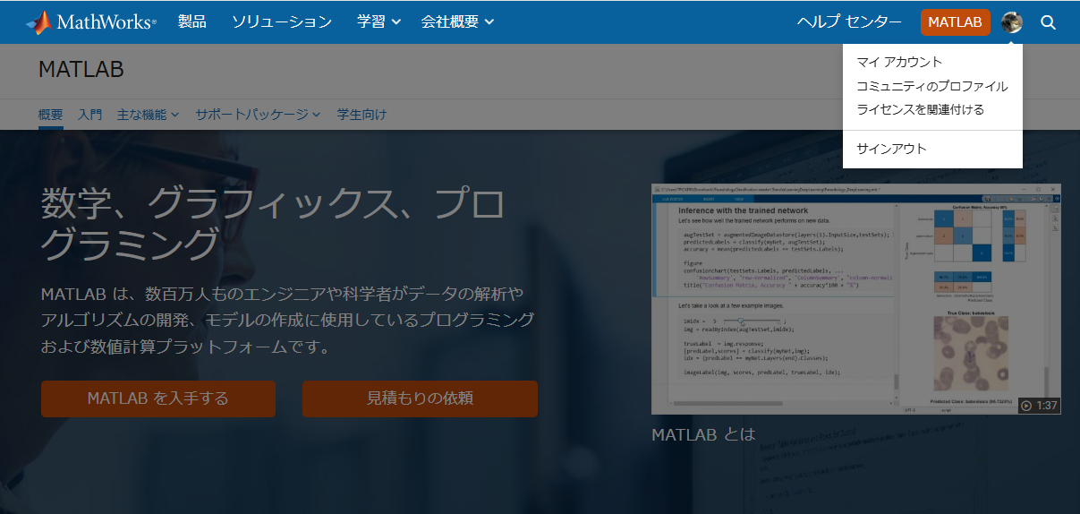
やっと表示される。気づかんって!
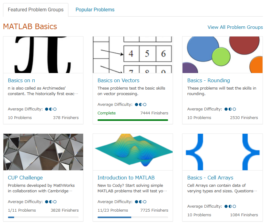
MATLAB Centralは無料で学べる宝物庫
とはいえ本当にオススメなんです。
どんなのがあるかさらっと紹介していきます。
ここは短い文章で問題を解くコードを書き上げるところ。
多様な分野を実践的に学ぶことができるし、何より他人のコードも見ることができる。
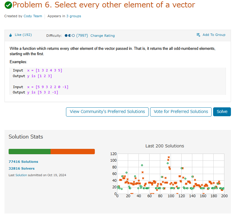
たまにそんなのありかよ~って回答もあるけどいい訓練になる。
ただ英語の問題見たらさ~ 悪い やっぱつれぇわ…
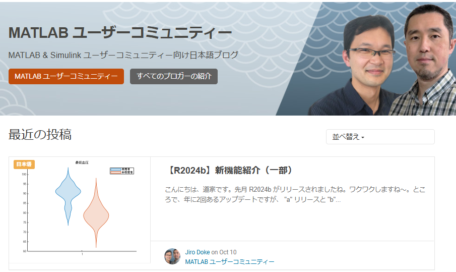
我らがアイドルmichioニキやJiro氏が新機能について紹介なんかもしてくれてる。
なんだかんだTwitter(現X)で紹介しちゃってるから、見るのさぼったり…ゲフンゲフン!
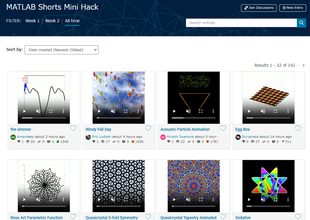
定期的に開催される。
プライズも貰えたりするし、何よりめっちゃ面白い作品を皆が書いてくる。
p=pi;
l = 5e3;
m = 0:l;
[u,v]=meshgrid(10*m/l*p,2*m/l*p);
c=cos(v/2);
s=sin(v);
e=1-exp(u/(6*p));
surf(2*e.*cos(u).*c.^2,-e*2.*sin(u).*c.^2,1-exp(u/(3.75*p))-s+exp(u/(5.5*p)).*s,'FaceColor','#a47a43','EdgeAlpha',0.02)
axis equal off
A=7.3;
zlim([-A 0])
view([-12 23])
set(gcf,'Color','#d2b071')

過去の事は水に流してくれないか?
toolboxにない自作関数とかを無料で皆が公開してるところ。
MATLABのアドオンからだと関数をそのままインストール出来たりする。
だいたいの答えはここにある。質問する前にググれば出てくる。
躓いて調べると過去に書いてあった自分の回答に助けられたりもする。
for文で回答すると一定数の海外ニキたちが
と絡んでくる。
Answersがバキバキ回答する場であるのに対して、ここでは好きなことを呟いていいらしい。最近できたっぽい。全然知らんかった。海外では「こんな機能欲しくね?」とかけっこう人気っぽい。
日本人が書いてないから僕がこんなクソスレ書いてるわけ┐(´д`)┌ヤレヤレ
まとめ
いかがだったでしょうか?このようにCentralは学びとして非常に有効な場所なのであります。インプットもいいけど是非アウトプットしてみましょう。コミュニティはアカウントさえ持ってたら無料でやれるんでね。
皆はどうやってMATLAB/Simulinkを学んだか、良ければ返信でクソレスしてくれると嬉しいです。特にSimulinkはマジでな~んにもわからん。MathWorksさんode45とかソルバーの説明ここでしてくれ。
後、ディスカッション一時保存機能つけてほしい。
最後に
Centralより先に、俺を救え
参考:ミスタードーナツを救え
If I go to a paint store, I can get foldout color charts/swatches for every brand of paint. I can make a selection and it will tell me the exact proportions of each of base color to add to a can of white paint. There doesn't seem to be any equivalent in MATLAB. The common word "swatch" doesn't even exist in the documentation. (?) One thinks pcolor() would be the way to go about this, but pcolor documentation is the most abstruse in all of the documentation. Thanks 1e+06 !
As pointed out in Doxygen comments in code generated with Simulink Embedded Coder - MATLAB Answers - MATLAB Central (mathworks.com), it would be nice that Embedded Coder has an option to generate Doxygen-style comments for signals of buses, i.e.:
/** @brief <Signal desciption here> **/
This would allow static analysis tools to parse the comments. Please add that feature!
As far as I know, starting from MATLAB R2024b, the documentation is defaulted to be accessed online. However, the problem is that every time I open the official online documentation through my browser, it defaults or forcibly redirects to the documentation hosted site for my current geographic location, often with multiple pop-up reminders, which is very annoying!
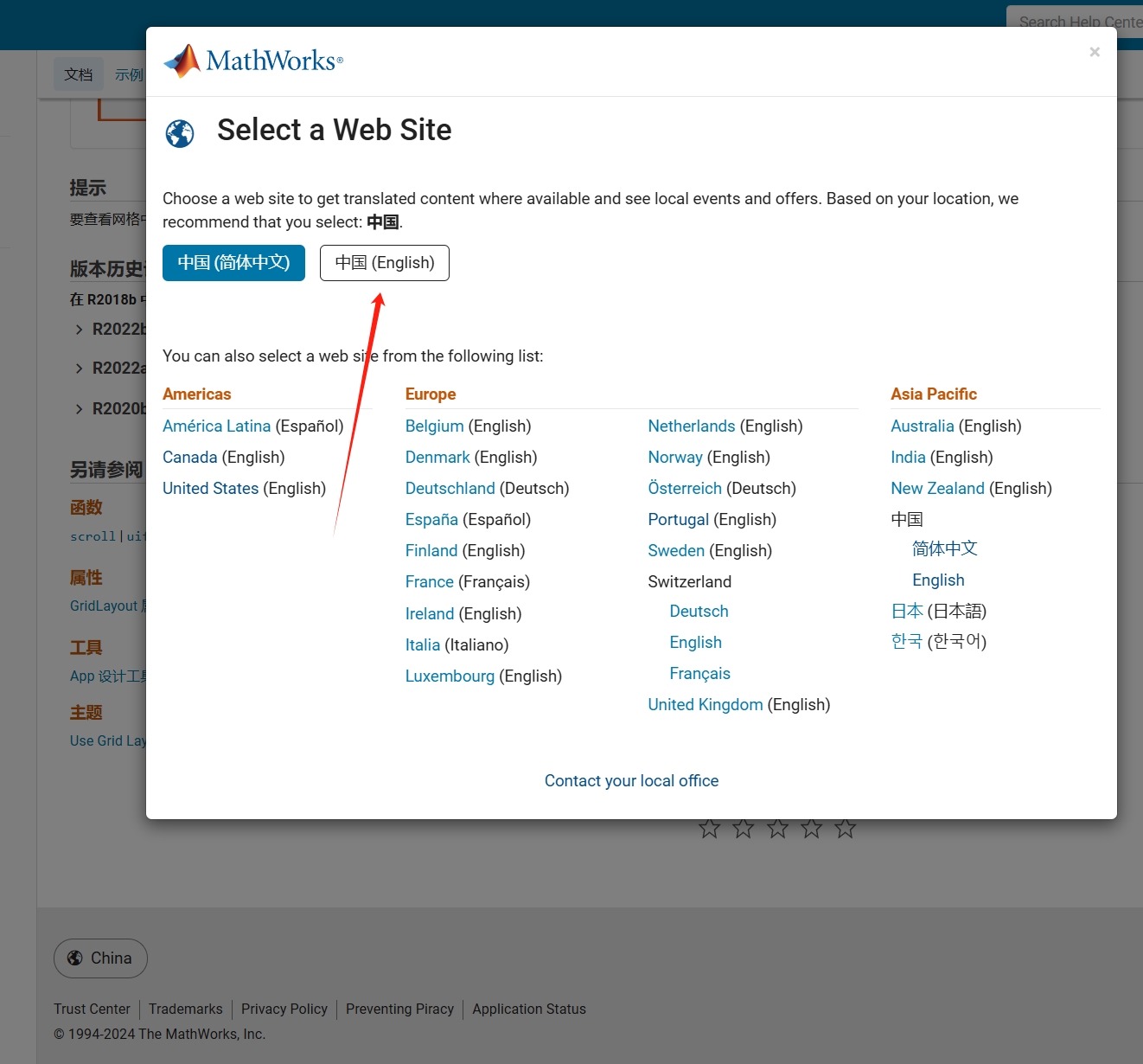
Suggestion: Could there be an option to set preferences linked to my personal account so that the documentation defaults to my chosen language preference without having to deal with “forced reminders” or “forced redirection” based on my geographic location? I prefer reading the English documentation, but the website automatically redirects me to the Chinese documentation due to my geolocation, which is quite frustrating!
----------------2024.12.13 update-----------------
Although the above issue was resolved by technical support, subsequent redirects are still causing severe delays...
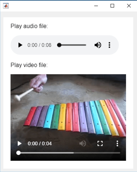
In the past two years, MATHWORKS has updated the image viewer and audio viewer, giving them a more modern interface with features like play, pause, fast forward, and some interactive tools that are more commonly found in typical third-party players. However, the video player has not seen any updates. For instance, the Video Viewer or vision.VideoPlayer could benefit from a more modern player interface. Perhaps I haven't found a suitable built-in player yet. It would be great if there were support for custom image processing and audio processing algorithms that could be played in a more modern interface in real time.
Additionally, I found it quite challenging to develop a modern video player from scratch in App Designer.(If there's a video component for that that would be great)
-----------------------------------------------------------------------------------------------------------------
BTW,the following picture shows the built-in function uihtml function showing a more modern playback interface with controls for play, pause and so on. But can not add real-time image processing algorithms within it.
isequaln exists to return true when NaN==NaN.
unique treats NaN==NaN as false (as it should) requiring NaN to be replaced if NaN is not considered unique in a particular application. In my application, I am checking uniqueness of table rows using [table_unique,index_unique]=unique(table,"rows","sorted") and would prefer to keep NaN as NaN or missing in table_unique without the overhead of replacing it with a dummy value then replacing it again. Dummy values also have the risk of matching existing values in the table, requiring first finding a dummy value that is not in the table.
uniquen (similar to isequaln) would be more eloquent.
Please point out if I am missing something!
Something that had bothered me ever since I became an FEA analyst (2012) was the apparent inability of the "camera" in Matlab's 3D plot to function like the "cameras" in CAD/CAE packages.
For instance, load the ForearmLink.stl model that ships with the PDE Toolbox in Matlab and ParaView and try rotating the model.
clear
close all
gm = importGeometry( "ForearmLink.stl" );
pdegplot(gm)
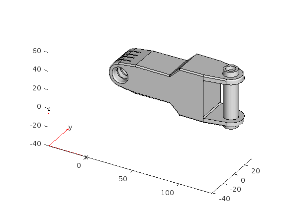
Things to observe:
- Note that I cant seem to rotate continuously around the x-axis. It appears to only support rotations from [0, 360] as opposed to [-inf, inf]. So, for example, if I'm looking in the Y+ direction and rotate around X so that I'm looking at the Z- direction, and then want to look in the Y- direction, I can't simply keep rotating around the X axis... instead have to rotate 180 degrees around the Z axis and then around the X axis. I'm not aware of any data visualization applications (e.g., ParaView, VisIt, EnSight) or CAD/CAE tools with such an interaction.
- Note that at the 50 second mark, I set a view in ParaView: looking in the [X-, Y-, Z-] direction with Y+ up. Try as I might in Matlab, I'm unable to achieve that same view perspective.
Today I discovered that if one turns on the Camera Toolbar from the View menubar, then clicks the Orbit Camera icon, then the No Principal Axis icon:
That then it acts in the manner I've long desired. Oh, and also, for the interested, it is programmatically available: https://www.mathworks.com/help/matlab/ref/cameratoolbar.html
I might humbly propose this mode either be made more discoverable, similar to the little interaction widgets that pop up in figures:
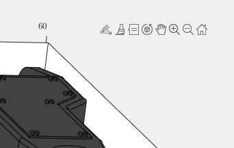
Or maybe use the middle-mouse button to temporarily use this mode (a mouse setting in, e.g., Abaqus/CAE).

I've noticed is that the highly rated fonts for coding (e.g. Fira Code, Inconsolata, etc.) seem to overlook one issue that is key for coding in Matlab. While these fonts make 0 and O, as well as the 1 and l easily distinguishable, the brackets are not. Quite often the curly bracket looks similar to the curved bracket, which can lead to mistakes when coding or reviewing code.
So I was thinking: Could Mathworks put together a team to review good programming fonts, and come up with their own custom font designed specifically and optimized for Matlab syntax?
An option for 10th degree polynomials but no weighted linear least squares. Seriously? Jesse
While searching the internet for some books on ordinary differential equations, I came across a link that I believe is very useful for all math students and not only. If you are interested in ODEs, it's worth taking the time to study it.
A First Look at Ordinary Differential Equations by Timothy S. Judson is an excellent resource for anyone looking to understand ODEs better. Here's a brief overview of the main topics covered:
- Introduction to ODEs: Basic concepts, definitions, and initial differential equations.
- Methods of Solution:
- Separable equations
- First-order linear equations
- Exact equations
- Transcendental functions
- Applications of ODEs: Practical examples and applications in various scientific fields.
- Systems of ODEs: Analysis and solutions of systems of differential equations.
- Series and Numerical Methods: Use of series and numerical methods for solving ODEs.
This book provides a clear and comprehensive introduction to ODEs, making it suitable for students and new researchers in mathematics. If you're interested, you can explore the book in more detail here: A First Look at Ordinary Differential Equations.
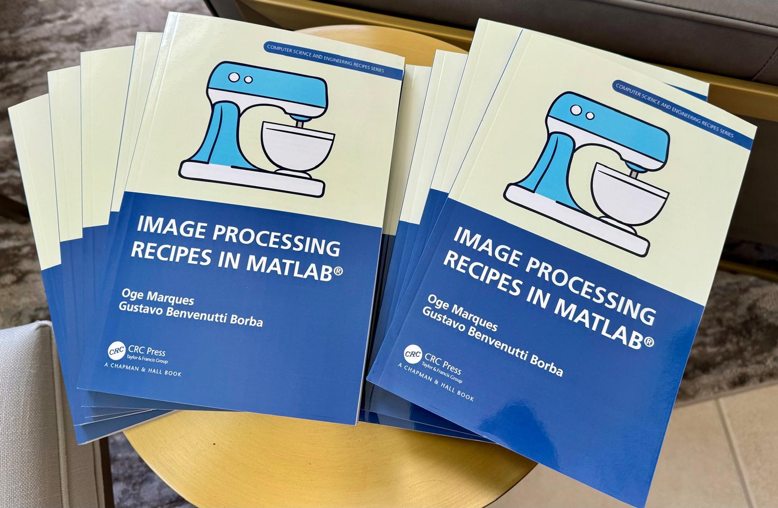
📚 New Book Announcement: "Image Processing Recipes in MATLAB" 📚
I am delighted to share the release of my latest book, "Image Processing Recipes in MATLAB," co-authored by my dear friend and colleague Gustavo Benvenutti Borba.
This 'cookbook' contains 30 practical recipes for image processing, ranging from foundational techniques to recently published algorithms. It serves as a concise and readable reference for quickly and efficiently deploying image processing pipelines in MATLAB.
Gustavo and I are immensely grateful to the MathWorks Book Program for their support. We also want to thank Randi Slack and her fantastic team at CRC Press for their patience, expertise, and professionalism throughout the process.
___________
A high school student called for help with this physics problem:
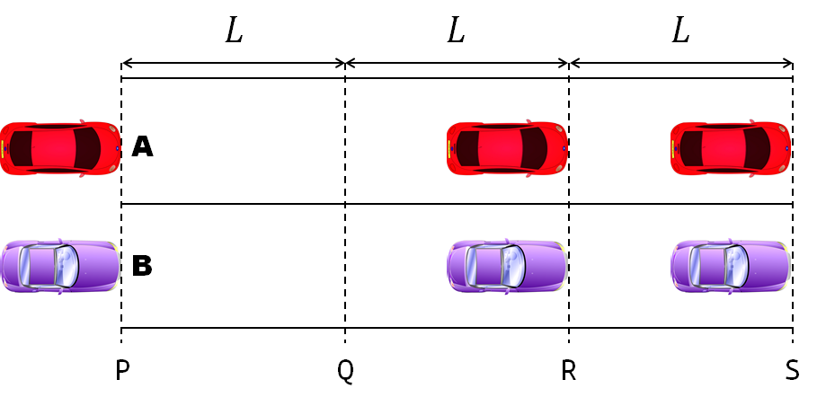
- Car A moves with constant velocity v.
- Car B starts to move when Car A passes through the point P.
- Car B undergoes...
- uniform acc. motion from P to Q.
- uniform velocity motion from Q to R.
- uniform acc. motion from R to S.
- Car A and B pass through the point R simultaneously.
- Car A and B arrive at the point S simultaneously.
Q1. When car A passes the point Q, which is moving faster?
Q2. Solve the time duration for car B to move from P to Q using L and v.
Q3. Magnitude of acc. of car B from P to Q, and from R to S: which is bigger?
Well, it can be solved with a series of tedious equations. But... how about this?
Code below:
%% get images and prepare stuffs
figure(WindowStyle="docked"),
ax1 = subplot(2,1,1);
hold on, box on
ax1.XTick = [];
ax1.YTick = [];
A = plot(0, 1, 'ro', MarkerSize=10, MarkerFaceColor='r');
B = plot(0, 0, 'bo', MarkerSize=10, MarkerFaceColor='b');
[carA, ~, alphaA] = imread('https://cdn.pixabay.com/photo/2013/07/12/11/58/car-145008_960_720.png');
[carB, ~, alphaB] = imread('https://cdn.pixabay.com/photo/2014/04/03/10/54/car-311712_960_720.png');
carA = imrotate(imresize(carA, 0.1), -90);
carB = imrotate(imresize(carB, 0.1), 180);
alphaA = imrotate(imresize(alphaA, 0.1), -90);
alphaB = imrotate(imresize(alphaB, 0.1), 180);
carA = imagesc(carA, AlphaData=alphaA, XData=[-0.1, 0.1], YData=[0.9, 1.1]);
carB = imagesc(carB, AlphaData=alphaB, XData=[-0.1, 0.1], YData=[-0.1, 0.1]);
txtA = text(0, 0.85, 'A', FontSize=12);
txtB = text(0, 0.17, 'B', FontSize=12);
yline(1, 'r--')
yline(0, 'b--')
xline(1, 'k--')
xline(2, 'k--')
text(1, -0.2, 'Q', FontSize=20, HorizontalAlignment='center')
text(2, -0.2, 'R', FontSize=20, HorizontalAlignment='center')
% legend('A', 'B') % this make the animation slow. why?
xlim([0, 3])
ylim([-.3, 1.3])
%% axes2: plots velocity graph
ax2 = subplot(2,1,2);
box on, hold on
xlabel('t'), ylabel('v')
vA = plot(0, 1, 'r.-');
vB = plot(0, 0, 'b.-');
xline(1, 'k--')
xline(2, 'k--')
xlim([0, 3])
ylim([-.3, 1.8])
p1 = patch([0, 0, 0, 0], [0, 1, 1, 0], [248, 209, 188]/255, ...
EdgeColor = 'none', ...
FaceAlpha = 0.3);
%% solution
v = 1; % car A moves with constant speed.
L = 1; % distances of P-Q, Q-R, R-S
% acc. of car B for three intervals
a(1) = 9*v^2/8/L;
a(2) = 0;
a(3) = -1;
t_BatQ = sqrt(2*L/a(1)); % time when car B arrives at Q
v_B2 = a(1) * t_BatQ; % speed of car B between Q-R
%% patches for velocity graph
p2 = patch([t_BatQ, t_BatQ, t_BatQ, t_BatQ], [1, 1, v_B2, v_B2], ...
[248, 209, 188]/255, ...
EdgeColor = 'none', ...
FaceAlpha = 0.3);
p3 = patch([2, 2, 2, 2], [1, v_B2, v_B2, 1], [194, 234, 179]/255, ...
EdgeColor = 'none', ...
FaceAlpha = 0.3);
%% animation
tt = linspace(0, 3, 2000);
for t = tt
A.XData = v * t;
vA.XData = [vA.XData, t];
vA.YData = [vA.YData, 1];
if t < t_BatQ
B.XData = 1/2 * a(1) * t^2;
vB.XData = [vB.XData, t];
vB.YData = [vB.YData, a(1) * t];
p1.XData = [0, t, t, 0];
p1.YData = [0, vB.YData(end), 1, 1];
elseif t >= t_BatQ && t < 2
B.XData = L + (t - t_BatQ) * v_B2;
vB.XData = [vB.XData, t];
vB.YData = [vB.YData, v_B2];
p2.XData = [t_BatQ, t, t, t_BatQ];
p2.YData = [1, 1, vB.YData(end), vB.YData(end)];
else
B.XData = 2*L + v_B2 * (t - 2) + 1/2 * a(3) * (t-2)^2;
vB.XData = [vB.XData, t];
vB.YData = [vB.YData, v_B2 + a(3) * (t - 2)];
p3.XData = [2, t, t, 2];
p3.YData = [1, 1, vB.YData(end), v_B2];
end
txtA.Position(1) = A.XData(end);
txtB.Position(1) = B.XData(end);
carA.XData = A.XData(end) + [-.1, .1];
carB.XData = B.XData(end) + [-.1, .1];
drawnow
end
Updating some of my educational Livescripts to 2024a, really love the new "define a function anywhere" feature, and have a "new" idea for improving Livescripts -- support "hidden" code blocks similar to the Jupyter Notebooks functionality.
For example, I often create "complicated" plots with a bunch of ancillary items and I don't want this code exposed to the reader by default, as it might confuse the reader. For example, consider a Livescript that might read like this:
-----
Noting the similar structure of these two mappings, let's now write a function that simply maps from some domain to some other domain using change of variable.
function x = ChangeOfVariable( x, from_domain, to_domain )
x = x - from_domain(1);
x = x * ( ( to_domain(2) - to_domain(1) ) / ( from_domain(2) - from_domain(1) ) );
x = x + to_domain(1);
end
Let's see this function in action
% HIDE CELL
clear
close all
from_domain = [-1, 1];
to_domain = [2, 7];
from_values = [-1, -0.5, 0, 0.5, 1];
to_values = ChangeOfVariable( from_values, from_domain, to_domain )
to_values = 1×5
2.0000 3.2500 4.5000 5.7500 7.0000
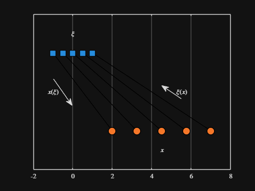
We can plot the values of from_values and to_values, showing how they're connected to each other:
% HIDE CELL
figure
hold on
for n = 1 : 5
plot( [from_values(n) to_values(n)], [1 0], Color="k", LineWidth=1 )
end
ax = gca;
ax.YTick = [];
ax.XLim = [ min( [from_domain, to_domain] ) - 1, max( [from_domain, to_domain] ) + 1 ];
ax.YLim = [-0.5, 1.5];
ax.XGrid = "on";
scatter( from_values, ones( 5, 1 ), Marker="s", MarkerFaceColor="flat", MarkerEdgeColor="k", SizeData=120, LineWidth=1, SeriesIndex=1 )
text( mean( from_domain ), 1.25, "$\xi$", Interpreter="latex", HorizontalAlignment="center", VerticalAlignment="middle" )
scatter( to_values, zeros( 5, 1 ), Marker="o", MarkerFaceColor="flat", MarkerEdgeColor="k", SizeData=120, LineWidth=1, SeriesIndex=2 )
text( mean( to_domain ), -0.25, "$x$", Interpreter="latex", HorizontalAlignment="center", VerticalAlignment="middle" )
scaled_arrow( ax, [mean( [from_domain(1), to_domain(1) ] ) - 1, 0.5], ( 1 - 0 ) / ( from_domain(1) - to_domain(1) ), 1 )
scaled_arrow( ax, [mean( [from_domain(end), to_domain(end)] ) + 1, 0.5], ( 1 - 0 ) / ( from_domain(end) - to_domain(end) ), -1 )
text( mean( [from_domain(1), to_domain(1) ] ) - 1.5, 0.5, "$x(\xi)$", Interpreter="latex", HorizontalAlignment="center", VerticalAlignment="middle" )
text( mean( [from_domain(end), to_domain(end)] ) + 1.5, 0.5, "$\xi(x)$", Interpreter="latex", HorizontalAlignment="center", VerticalAlignment="middle" )
-----
Where scaled_arrow is some utility function I've defined elsewhere... See how a majority of the code is simply "drivel" to create the plot, clear and close? I'd like to be able to hide those cells so that it would look more like this:
-----
Noting the similar structure of these two mappings, let's now write a function that simply maps from some domain to some other domain using change of variable.
function x = ChangeOfVariable( x, from_domain, to_domain )
x = x - from_domain(1);
x = x * ( ( to_domain(2) - to_domain(1) ) / ( from_domain(2) - from_domain(1) ) );
x = x + to_domain(1);
end
Let's see this function in action
▶ Show code cell
from_domain = [-1, 1];
to_domain = [2, 7];
from_values = [-1, -0.5, 0, 0.5, 1];
to_values = ChangeOfVariable( from_values, from_domain, to_domain )
to_values = 1×5
2.0000 3.2500 4.5000 5.7500 7.0000
We can plot the values of from_values and to_values, showing how they're connected to each other:
▶ Show code cell

-----
Thoughts?
Seleziona un sito web
Seleziona un sito web per visualizzare contenuto tradotto dove disponibile e vedere eventi e offerte locali. In base alla tua area geografica, ti consigliamo di selezionare: United States.
Puoi anche selezionare un sito web dal seguente elenco:
Americhe
- América Latina (Español)
- Canada (English)
- United States (English)
Europa
- Belgium (English)
- Denmark (English)
- Deutschland (Deutsch)
- España (Español)
- Finland (English)
- France (Français)
- Ireland (English)
- Italia (Italiano)
- Luxembourg (English)
- Netherlands (English)
- Norway (English)
- Österreich (Deutsch)
- Portugal (English)
- Sweden (English)
- Switzerland
- United Kingdom (English)