Risultati per
I am deeply honored to announce the official publication of my latest academic volume:
MATLAB for Civil Engineers: From Basics to Advanced Applications
(Springer Nature, 2025).
This work serves as a comprehensive bridge between theoretical civil engineering principles and their practical implementation through MATLAB—a platform essential to the future of computational design, simulation, and optimization in our field.
Structured to serve both academic audiences and practicing engineers, this book progresses from foundational MATLAB programming concepts to highly specialized applications in structural analysis, geotechnical engineering, hydraulic modeling, and finite element methods. Whether you are a student building analytical fluency or a professional seeking computational precision, this volume offers an indispensable resource for mastering MATLAB's full potential in civil engineering contexts.
With rigorously structured examples, case studies, and research-aligned methods, MATLAB for Civil Engineers reflects the convergence of engineering logic with algorithmic innovation—equipping readers to address contemporary challenges with clarity, accuracy, and foresight.
📖 Ideal for:
— Graduate and postgraduate civil engineering students
— University instructors and lecturers seeking a structured teaching companion
— Professionals aiming to integrate MATLAB into complex real-world projects
If you are passionate about engineering resilience, data-informed design, or computational modeling, I invite you to explore the work and share it with your network.
🧠 Let us advance the discipline together through precision, programming, and purpose.

Los invito a conocer el libro "Sistemas dinámicos en contexto: Modelación matemática, simulación, estimación y control con MATLAB", el cual ya está disponible en formato digital.
El libro integra diversos temas de los sistemas dinámicos desde un punto de vista práctico utilizando programas de MATLAB y simulaciones en Simulink y utilizando métodos numéricos (ver enlace). Existe mucho material en el blog del libro con posibilidades para comentarios, propuestas y correcciones. Resalto los casos de estudio
Creo que el libro les puede dar un buen panorama del área con la posibilidad de experimentar de manera interactiva con todo el material de MATLAB disponible en formato Live Script. Lo mejor es que se pueden formular preguntas en el blog y hacer propuestas al autor de ejercicios resueltos.
Son bienvenidos los comentarios, sugerencias y correcciones al texto.
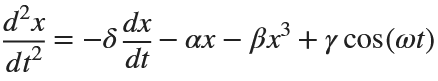
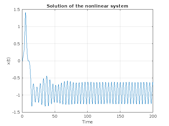
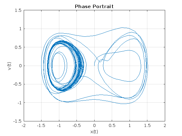
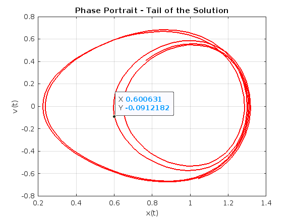
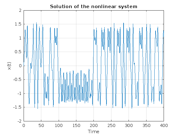
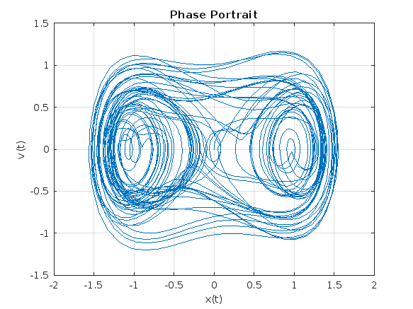
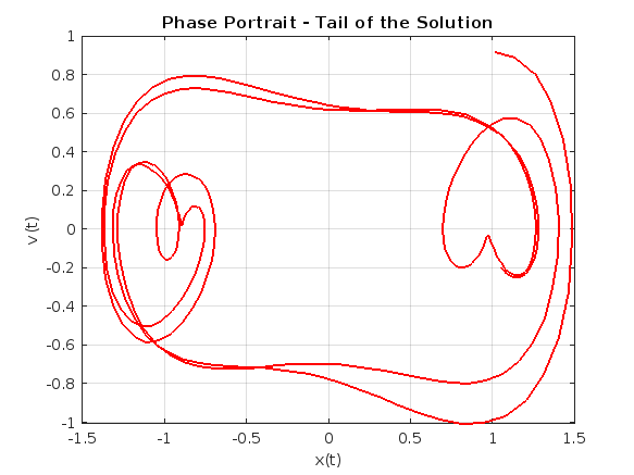
Following on from my previous post The Non-Chaotic Duffing Equation, now we will study the chaotic behaviour of the Duffing Equation
P.s:Any comments/advice on improving the code is welcome.
The Original Duffing Equation is the following:
Let 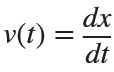 . This implies that
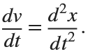
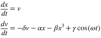
Then we rewrite it as a System of First-Order Equations
Using the substitution  for
for  , the second-order equation can be transformed into the following system of first-order equations:
Exploring the Effect of γ.
% Define parameters
gamma = 0.1;
alpha = -1;
beta = 1;
delta = 0.1;
omega = 1.4;
% Define the system of equations
odeSystem = @(t, y) [y(2);
-delta*y(2) - alpha*y(1) - beta*y(1)^3 + gamma*cos(omega*t)];
% Initial conditions
y0 = [0; 0]; % x(0) = 0, v(0) = 0
% Time span
tspan = [0 200];
% Solve the system
[t, y] = ode45(odeSystem, tspan, y0);
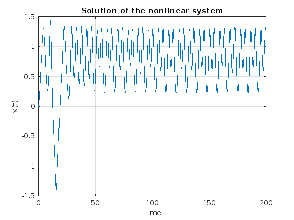
% Plot the results
figure;
plot(t, y(:, 1));
xlabel('Time');
ylabel('x(t)');
title('Solution of the nonlinear system');
grid on;
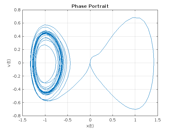
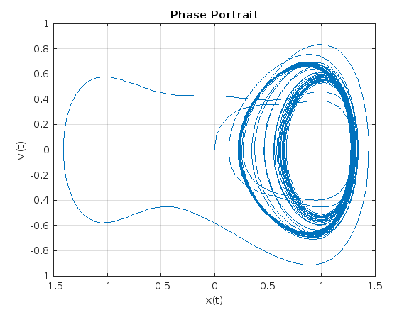
% Plot the phase portrait
figure;
plot(y(:, 1), y(:, 2));
xlabel('x(t)');
ylabel('v(t)');
title('Phase Portrait');
grid on;
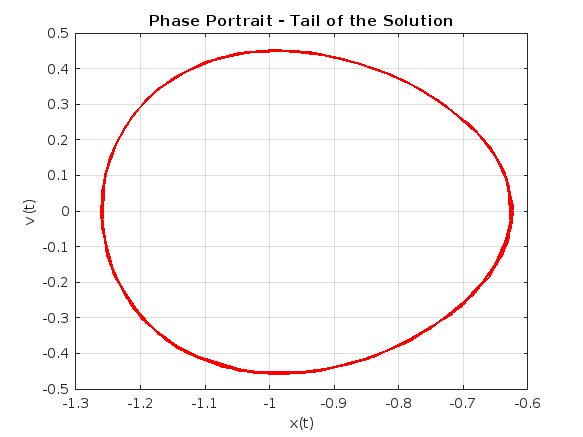
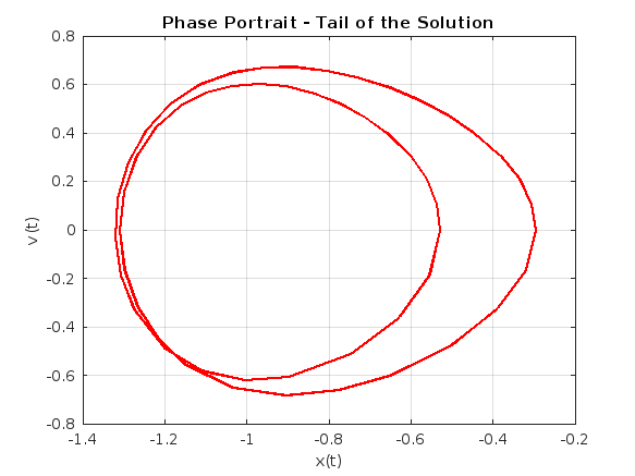
% Define the tail (e.g., last 10% of the time interval)
tail_start = floor(0.9 * length(t)); % Starting index for the tail
tail_end = length(t); % Ending index for the tail
% Plot the tail of the solution
figure;
plot(y(tail_start:tail_end, 1), y(tail_start:tail_end, 2), 'r', 'LineWidth', 1.5);
xlabel('x(t)');
ylabel('v(t)');
title('Phase Portrait - Tail of the Solution');
grid on;
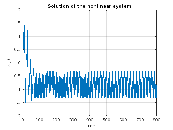
% Define parameters
gamma = 0.318;
alpha = -1;
beta = 1;
delta = 0.1;
omega = 1.4;
% Define the system of equations
odeSystem = @(t, y) [y(2);
-delta*y(2) - alpha*y(1) - beta*y(1)^3 + gamma*cos(omega*t)];
% Initial conditions
y0 = [0; 0]; % x(0) = 0, v(0) = 0
% Time span
tspan = [0 800];
% Solve the system
[t, y] = ode45(odeSystem, tspan, y0);
% Plot the results
figure;
plot(t, y(:, 1));
xlabel('Time');
ylabel('x(t)');
title('Solution of the nonlinear system');
grid on;
% Plot the phase portrait
figure;
plot(y(:, 1), y(:, 2));
xlabel('x(t)');
ylabel('v(t)');
title('Phase Portrait');
grid on;
% Define the tail (e.g., last 10% of the time interval)
tail_start = floor(0.9 * length(t)); % Starting index for the tail
tail_end = length(t); % Ending index for the tail
% Plot the tail of the solution
figure;
plot(y(tail_start:tail_end, 1), y(tail_start:tail_end, 2), 'r', 'LineWidth', 1.5);
xlabel('x(t)');
ylabel('v(t)');
title('Phase Portrait - Tail of the Solution');
grid on;
% Define parameters
gamma = 0.338;
alpha = -1;
beta = 1;
delta = 0.1;
omega = 1.4;
% Define the system of equations
odeSystem = @(t, y) [y(2);
-delta*y(2) - alpha*y(1) - beta*y(1)^3 + gamma*cos(omega*t)];
% Initial conditions
y0 = [0; 0]; % x(0) = 0, v(0) = 0
% Time span with more points for better resolution
tspan = linspace(0, 200,2000); % Increase the number of points
% Solve the system
[t, y] = ode45(odeSystem, tspan, y0);
% Plot the results
figure;
plot(t, y(:, 1));
xlabel('Time');
ylabel('x(t)');
title('Solution of the nonlinear system');
grid on;
% Plot the phase portrait
figure;
plot(y(:, 1), y(:, 2));
xlabel('x(t)');
ylabel('v(t)');
title('Phase Portrait');
grid on;
% Define the tail (e.g., last 10% of the time interval)
tail_start = floor(0.9 * length(t)); % Starting index for the tail
tail_end = length(t); % Ending index for the tail
% Plot the tail of the solution
figure;
plot(y(tail_start:tail_end, 1), y(tail_start:tail_end, 2), 'r', 'LineWidth', 1.5);
xlabel('x(t)');
ylabel('v(t)');
title('Phase Portrait - Tail of the Solution');
grid on;
ax = gca;
chart = ax.Children(1);
datatip(chart,0.5581,-0.1126);
% Define parameters
gamma = 0.35;
alpha = -1;
beta = 1;
delta = 0.1;
omega = 1.4;
% Define the system of equations
odeSystem = @(t, y) [y(2);
-delta*y(2) - alpha*y(1) - beta*y(1)^3 + gamma*cos(omega*t)];
% Initial conditions
y0 = [0; 0]; % x(0) = 0, v(0) = 0
% Time span with more points for better resolution
tspan = linspace(0, 400,3000); % Increase the number of points
% Solve the system
[t, y] = ode45(odeSystem, tspan, y0);
% Plot the results
figure;
plot(t, y(:, 1));
xlabel('Time');
ylabel('x(t)');
title('Solution of the nonlinear system');
grid on;
% Plot the phase portrait
figure;
plot(y(:, 1), y(:, 2));
xlabel('x(t)');
ylabel('v(t)');
title('Phase Portrait');
grid on;
% Define the tail (e.g., last 10% of the time interval)
tail_start = floor(0.9 * length(t)); % Starting index for the tail
tail_end = length(t); % Ending index for the tail
% Plot the tail of the solution
figure;
plot(y(tail_start:tail_end, 1), y(tail_start:tail_end, 2), 'r', 'LineWidth', 1.5);
xlabel('x(t)');
ylabel('v(t)');
title('Phase Portrait - Tail of the Solution');
grid on;
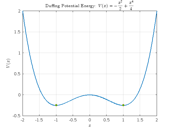
Studying the attached document Duffing Equation from the University of Colorado, I noticed that there is an analysis of The Non-Chaotic Duffing Equation and all the graphs were created with Matlab. And since the code is not given I took the initiative to try to create the same graphs with the following code.
- Plotting the Potential Energy and Identifying Extrema
% Define the range of x values
x = linspace(-2, 2, 1000);
% Define the potential function V(x)
V = -x.^2 / 2 + x.^4 / 4;
% Plot the potential function
figure;
plot(x, V, 'LineWidth', 2);
hold on;
% Mark the minima at x = ±1
plot([-1, 1], [-1/4, -1/4], 'ro', 'MarkerSize', 5, 'MarkerFaceColor', 'g');
% Add LaTeX title and labels
title('Duffing Potential Energy: $$V(x) = -\frac{x^2}{2} + \frac{x^4}{4}$$', 'Interpreter', 'latex');
xlabel('$$x$$', 'Interpreter', 'latex');
ylabel('$$V(x)$$','Interpreter', 'latex');
grid on;
hold off;
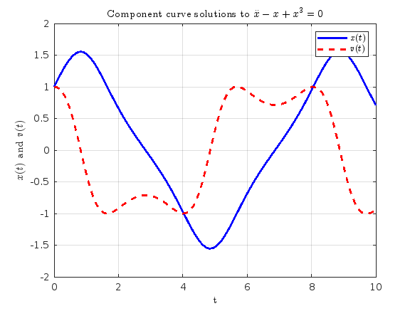
- Solving and Plotting the Duffing Equation
% Define the system of ODEs for the non-chaotic Duffing equation
duffing_ode = @(t, X) [X(2);
X(1) - X(1).^3];
% Time span for the simulation
tspan = [0 10];
% Initial conditions [x(0), v(0)]
initial_conditions = [1; 1];
% Solve the ODE using ode45
[t, X] = ode45(duffing_ode, tspan, initial_conditions);
% Extract displacement (x) and velocity (v)
x = X(:, 1);
v = X(:, 2);
% Plot both x(t) and v(t) in the same figure
figure;
plot(t, x, 'b-', 'LineWidth', 2); % Plot x(t) with blue line
hold on;
plot(t, v, 'r--', 'LineWidth', 2); % Plot v(t) with red dashed line
% Add title, labels, and legend
title(' Component curve solutions to $$\ddot{x}-x+x^3=0$$','Interpreter', 'latex');
xlabel('t','Interpreter', 'latex');
ylabel('$$x(t) $$ and $$v(t) $$','Interpreter', 'latex');
legend('$$x(t)$$', ' $$v(t)$$','Interpreter', 'latex');
grid on;
hold off;
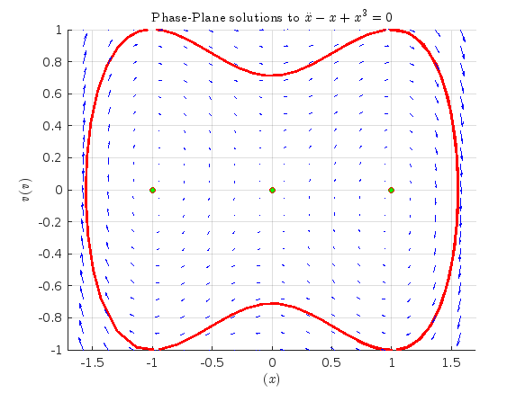
% Phase portrait with nullclines, equilibria, and vector field
figure;
hold on;
% Plot phase portrait
plot(x, v,'r', 'LineWidth', 2);
% Plot equilibrium points
plot([0 1 -1], [0 0 0], 'ro', 'MarkerSize', 5, 'MarkerFaceColor', 'g');
% Create a grid of points for the vector field
[x_vals, v_vals] = meshgrid(linspace(-2, 2, 20), linspace(-1, 1, 20));
% Compute the vector field components
dxdt = v_vals;
dvdt = x_vals - x_vals.^3;
% Plot the vector field
quiver(x_vals, v_vals, dxdt, dvdt, 'b');
% Set axis limits to [-1, 1]
xlim([-1.7 1.7]);
ylim([-1 1]);
% Labels and title
title('Phase-Plane solutions to $$\ddot{x}-x+x^3=0$$','Interpreter', 'latex');
xlabel('$$ (x)$$','Interpreter', 'latex');
ylabel('$$v(v)$$','Interpreter', 'latex');
grid on;
hold off;
An attractor is called strange if it has a fractal structure, that is if it has non-integer Hausdorff dimension. This is often the case when the dynamics on it are chaotic, but strange nonchaotic attractors also exist. If a strange attractor is chaotic, exhibiting sensitive dependence on initial conditions, then any two arbitrarily close alternative initial points on the attractor, after any of various numbers of iterations, will lead to points that are arbitrarily far apart (subject to the confines of the attractor), and after any of various other numbers of iterations will lead to points that are arbitrarily close together. Thus a dynamic system with a chaotic attractor is locally unstable yet globally stable: once some sequences have entered the attractor, nearby points diverge from one another but never depart from the attractor.
The term strange attractor was coined by David Ruelle and Floris Takens to describe the attractor resulting from a series of bifurcations of a system describing fluid flow. Strange attractors are often differentiable in a few directions, but some are like a Cantor dust, and therefore not differentiable. Strange attractors may also be found in the presence of noise, where they may be shown to support invariant random probability measures of Sinai–Ruelle–Bowen type.
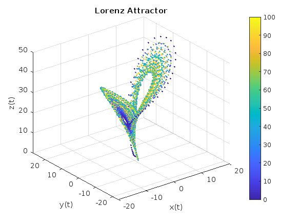
Lorenz
% Lorenz Attractor Parameters
sigma = 10;
beta = 8/3;
rho = 28;
% Lorenz system of differential equations
f = @(t, a) [-sigma*a(1) + sigma*a(2);
rho*a(1) - a(2) - a(1)*a(3);
-beta*a(3) + a(1)*a(2)];
% Time span
tspan = [0 100];
% Initial conditions
a0 = [1 1 1];
% Solve the system using ode45
[t, a] = ode45(f, tspan, a0);
% Plot using scatter3 with time-based color mapping
figure;
scatter3(a(:,1), a(:,2), a(:,3), 5, t, 'filled'); % 5 is the marker size
title('Lorenz Attractor');
xlabel('x(t)');
ylabel('y(t)');
zlabel('z(t)');
grid on;
colorbar; % Add a colorbar to indicate the time mapping
view(3); % Set the view to 3D
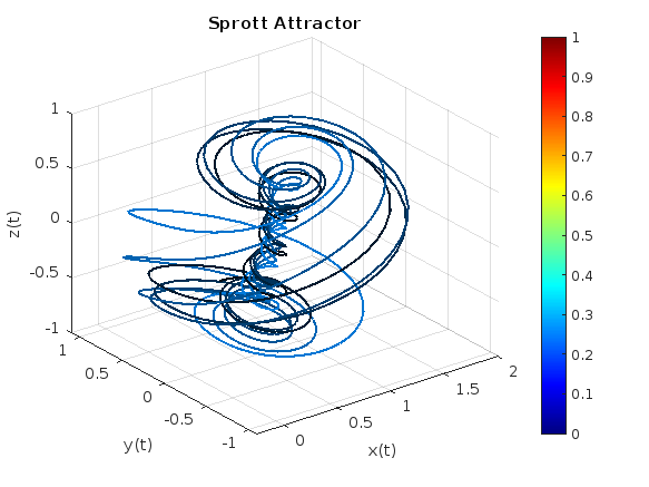
Sprott
% Define the parameters
a = 2.07;
b = 1.79;
% Define the system of differential equations
dynamics = @(t, X) [ ...
X(2) + a * X(1) * X(2) + X(1) * X(3); % dx/dt
1 - b * X(1)^2 + X(2) * X(3); % dy/dt
X(1) - X(1)^2 - X(2)^2 % dz/dt
];
% Initial conditions
X0 = [0.63; 0.47; -0.54];
% Time span
tspan = [0 100];
% Solve the system using ode45
[t, X] = ode45(dynamics, tspan, X0);
% Plot the results with color gradient
figure;
colormap(jet); % Set the colormap
c = linspace(1, 10, length(t)); % Color data based on time
% Create a 3D line plot with color based on time
for i = 1:length(t)-1
plot3(X(i:i+1,1), X(i:i+1,2), X(i:i+1,3), 'Color', [0 0.5 0.9]*c(i)/10, 'LineWidth', 1.5);
hold on;
end
% Set plot properties
title('Sprott Attractor');
xlabel('x(t)');
ylabel('y(t)');
zlabel('z(t)');
grid on;
colorbar; % Add a colorbar to indicate the time mapping
view(3); % Set the view to 3D
hold off;
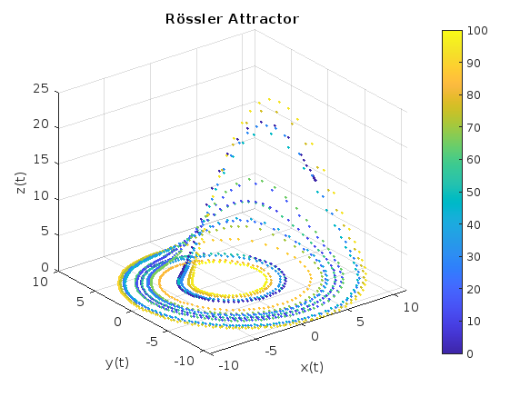
Rössler
% Define the parameters
a = 0.2;
b = 0.2;
c = 5.7;
% Define the system of differential equations
dynamics = @(t, X) [ ...
-(X(2) + X(3)); % dx/dt
X(1) + a * X(2); % dy/dt
b + X(3) * (X(1) - c) % dz/dt
];
% Initial conditions
X0 = [10.0; 0.00; 10.0];
% Time span
tspan = [0 100];
% Solve the system using ode45
[t, X] = ode45(dynamics, tspan, X0);
% Plot the results
figure;
scatter3(X(:,1), X(:,2), X(:,3), 5, t, 'filled');
title('Rössler Attractor');
xlabel('x(t)');
ylabel('y(t)');
zlabel('z(t)');
grid on;
colorbar; % Add a colorbar to indicate the time mapping
view(3); % Set the view to 3D
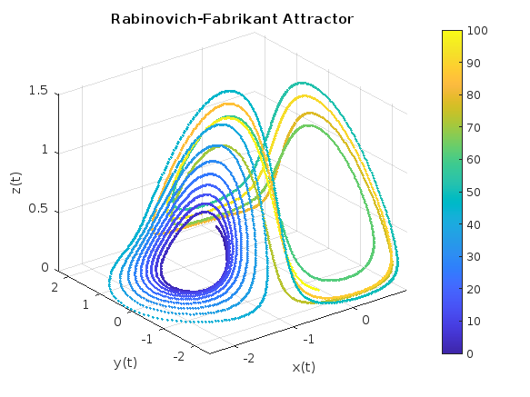
Rabinovich-Fabrikant
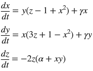
%% Parameters for Rabinovich-Fabrikant Attractor
alpha = 0.14;
gamma = 0.10;
dt = 0.01;
num_steps = 5000;
% Initial conditions
x0 = -1;
y0 = 0;
z0 = 0.5;
% Preallocate arrays for performance
x = zeros(1, num_steps);
y = zeros(1, num_steps);
z = zeros(1, num_steps);
% Set initial values
x(1) = x0;
y(1) = y0;
z(1) = z0;
% Generate the attractor
for i = 1:num_steps-1
x(i+1) = x(i) + dt * (y(i)*(z(i) - 1 + x(i)^2) + gamma*x(i));
y(i+1) = y(i) + dt * (x(i)*(3*z(i) + 1 - x(i)^2) + gamma*y(i));
z(i+1) = z(i) + dt * (-2*z(i)*(alpha + x(i)*y(i)));
end
% Create a time vector for color mapping
t = linspace(0, 100, num_steps);
% Plot using scatter3
figure;
scatter3(x, y, z, 5, t, 'filled'); % 5 is the marker size
title('Rabinovich-Fabrikant Attractor');
xlabel('x(t)');
ylabel('y(t)');
zlabel('z(t)');
grid on;
colorbar; % Add a colorbar to indicate the time mapping
view(3); % Set the view to 3D
References
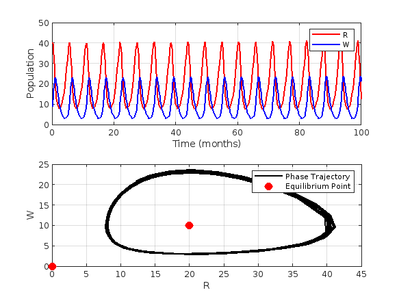
This project discusses predator-prey system, particularly the Lotka-Volterra equations,which model the interaction between two sprecies: prey and predators. Let's solve the Lotka-Volterra equations numerically and visualize the results.% Define parameters
% Define parameters
alpha = 1.0; % Prey birth rate
beta = 0.1; % Predator success rate
gamma = 1.5; % Predator death rate
delta = 0.075; % Predator reproduction rate
% Define the symbolic variables
syms R W
% Define the equations
eq1 = alpha * R - beta * R * W == 0;
eq2 = delta * R * W - gamma * W == 0;
% Solve the equations
equilibriumPoints = solve([eq1, eq2], [R, W]);
% Extract the equilibrium point values
Req = double(equilibriumPoints.R);
Weq = double(equilibriumPoints.W);
% Display the equilibrium points
equilibriumPointsValues = [Req, Weq]
% Solve the differential equations using ode45
lotkaVolterra = @(t,Y)[alpha*Y(1)-beta*Y(1)*Y(2);
delta*Y(1)*Y(2)-gamma*Y(2)];
% Initial conditions
R0 = 40;
W0 = 9;
Y0 = [R0, W0];
tspan = [0, 100];
% Solve the differential equations
[t, Y] = ode45(lotkaVolterra, tspan, Y0);
% Extract the populations
R = Y(:, 1);
W = Y(:, 2);
% Plot the results
figure;
subplot(2,1,1);
plot(t, R, 'r', 'LineWidth', 1.5);
hold on;
plot(t, W, 'b', 'LineWidth', 1.5);
xlabel('Time (months)');
ylabel('Population');
legend('R', 'W');
grid on;
subplot(2,1,2);
plot(R, W, 'k', 'LineWidth', 1.5);
xlabel('R');
ylabel('W');
grid on;
hold on;
plot(Req, Weq, 'ro', 'MarkerSize', 8, 'MarkerFaceColor', 'r');
legend('Phase Trajectory', 'Equilibrium Point');
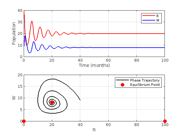
Now, we need to handle a modified version of the Lotka-Volterra equations. These modified equations incorporate logistic growth fot the prey population.
These equations are:
% Define parameters
alpha = 1.0;
K = 100; % Carrying Capacity of the prey population
beta = 0.1;
gamma = 1.5;
delta = 0.075;
% Define the symbolic variables
syms R W
% Define the equations
eq1 = alpha*R*(1 - R/K) - beta*R*W == 0;
eq2 = delta*R*W - gamma*W == 0;
% Solve the equations
equilibriumPoints = solve([eq1, eq2], [R, W]);
% Extract the equilibrium point values
Req = double(equilibriumPoints.R);
Weq = double(equilibriumPoints.W);
% Display the equilibrium points
equilibriumPointsValues = [Req, Weq]
% Solve the differential equations using ode45
modified_lv = @(t,Y)[alpha*Y(1)*(1-Y(1)/K)-beta*Y(1)*Y(2);
delta*Y(1)*Y(2)-gamma*Y(2)];
% Initial conditions
R0 = 40;
W0 = 9;
Y0 = [R0, W0];
tspan = [0, 100];
% Solve the differential equations
[t, Y] = ode45(modified_lv, tspan, Y0);
% Extract the populations
R = Y(:, 1);
W = Y(:, 2);
% Plot the results
figure;
subplot(2,1,1);
plot(t, R, 'r', 'LineWidth', 1.5);
hold on;
plot(t, W, 'b', 'LineWidth', 1.5);
xlabel('Time (months)');
ylabel('Population');
legend('R', 'W');
grid on;
subplot(2,1,2);
plot(R, W, 'k', 'LineWidth', 1.5);
xlabel('R');
ylabel('W');
grid on;
hold on;
plot(Req, Weq, 'ro', 'MarkerSize', 8, 'MarkerFaceColor', 'r');
legend('Phase Trajectory', 'Equilibrium Point');
While searching the internet for some books on ordinary differential equations, I came across a link that I believe is very useful for all math students and not only. If you are interested in ODEs, it's worth taking the time to study it.
A First Look at Ordinary Differential Equations by Timothy S. Judson is an excellent resource for anyone looking to understand ODEs better. Here's a brief overview of the main topics covered:
- Introduction to ODEs: Basic concepts, definitions, and initial differential equations.
- Methods of Solution:
- Separable equations
- First-order linear equations
- Exact equations
- Transcendental functions
- Applications of ODEs: Practical examples and applications in various scientific fields.
- Systems of ODEs: Analysis and solutions of systems of differential equations.
- Series and Numerical Methods: Use of series and numerical methods for solving ODEs.
This book provides a clear and comprehensive introduction to ODEs, making it suitable for students and new researchers in mathematics. If you're interested, you can explore the book in more detail here: A First Look at Ordinary Differential Equations.
The study of the dynamics of the discrete Klein - Gordon equation (DKG) with friction is given by the equation :

In the above equation, W describes the potential function: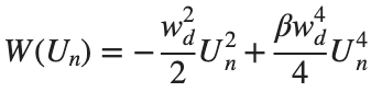
to which every coupled unit  adheres. In Eq. (1), the variable $
 $ is the unknown displacement of the oscillator occupying the n-th position of the lattice, and
  is the discretization parameter. We denote by h the distance between the oscillators of the lattice. The chain (DKG) contains linear damping with a damping coefficient
  , while
 is the coefficient of the nonlinear cubic term.
$ is the unknown displacement of the oscillator occupying the n-th position of the lattice, and For the DKG chain (1), we will consider the problem of initial-boundary values, with initial conditions

and Dirichlet boundary conditions at the boundary points  and
and  , that is,
and , that is,
Therefore, when necessary, we will use the short notation  for the one-dimensional discrete Laplacian
for the one-dimensional discrete Laplacian
Now we want to investigate numerically the dynamics of the system (1)-(2)-(3). Our first aim is to conduct a numerical study of the property of Dynamic Stability of the system, which directly depends on the existence and linear stability of the branches of equilibrium points.
For the discussion of numerical results, it is also important to emphasize the role of the parameter  . By changing the time variable
  , we rewrite Eq. (1) in the form
 . We consider spatially extended initial conditions of the form:
We also assume zero initial velocity:
the following graphs for  and
and 
% Parameters
L = 200; % Length of the system
K = 99; % Number of spatial points
j = 2; % Mode number
omega_d = 1; % Characteristic frequency
beta = 1; % Nonlinearity parameter
delta = 0.05; % Damping coefficient
% Spatial grid
h = L / (K + 1);
n = linspace(-L/2, L/2, K+2); % Spatial points
N = length(n);
omegaDScaled = h * omega_d;
deltaScaled = h * delta;
% Time parameters
dt = 1; % Time step
tmax = 3000; % Maximum time
tspan = 0:dt:tmax; % Time vector
% Values of amplitude 'a' to iterate over
a_values = [2, 1.95, 1.9, 1.85, 1.82]; % Modify this array as needed
% Differential equation solver function
function dYdt = odefun(~, Y, N, h, omegaDScaled, deltaScaled, beta)
U = Y(1:N);
Udot = Y(N+1:end);
Uddot = zeros(size(U));
% Laplacian (discrete second derivative)
for k = 2:N-1
Uddot(k) = (U(k+1) - 2 * U(k) + U(k-1)) ;
end
% System of equations
dUdt = Udot;
dUdotdt = Uddot - deltaScaled * Udot + omegaDScaled^2 * (U - beta * U.^3);
% Pack derivatives
dYdt = [dUdt; dUdotdt];
end
% Create a figure for subplots
figure;
% Initial plot
a_init = 2; % Example initial amplitude for the initial condition plot
U0_init = a_init * sin((j * pi * h * n) / L); % Initial displacement
U0_init(1) = 0; % Boundary condition at n = 0
U0_init(end) = 0; % Boundary condition at n = K+1
subplot(3, 2, 1);
plot(n, U0_init, 'r.-', 'LineWidth', 1.5, 'MarkerSize', 10); % Line and marker plot
xlabel('$x_n$', 'Interpreter', 'latex');
ylabel('$U_n$', 'Interpreter', 'latex');
title('$t=0$', 'Interpreter', 'latex');
set(gca, 'FontSize', 12, 'FontName', 'Times');
xlim([-L/2 L/2]);
ylim([-3 3]);
grid on;
% Loop through each value of 'a' and generate the plot
for i = 1:length(a_values)
a = a_values(i);
% Initial conditions
U0 = a * sin((j * pi * h * n) / L); % Initial displacement
U0(1) = 0; % Boundary condition at n = 0
U0(end) = 0; % Boundary condition at n = K+1
Udot0 = zeros(size(U0)); % Initial velocity
% Pack initial conditions
Y0 = [U0, Udot0];
% Solve ODE
opts = odeset('RelTol', 1e-5, 'AbsTol', 1e-6);
[t, Y] = ode45(@(t, Y) odefun(t, Y, N, h, omegaDScaled, deltaScaled, beta), tspan, Y0, opts);
% Extract solutions
U = Y(:, 1:N);
Udot = Y(:, N+1:end);
% Plot final displacement profile
subplot(3, 2, i+1);
plot(n, U(end,:), 'b.-', 'LineWidth', 1.5, 'MarkerSize', 10); % Line and marker plot
xlabel('$x_n$', 'Interpreter', 'latex');
ylabel('$U_n$', 'Interpreter', 'latex');
title(['$t=3000$, $a=', num2str(a), '$'], 'Interpreter', 'latex');
set(gca, 'FontSize', 12, 'FontName', 'Times');
xlim([-L/2 L/2]);
ylim([-2 2]);
grid on;
end
% Adjust layout
set(gcf, 'Position', [100, 100, 1200, 900]); % Adjust figure size as needed
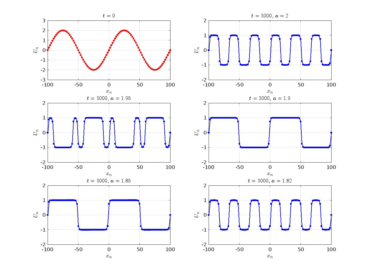
Dynamics for the initial condition ,  , for
, for  , for different amplitude values. By reducing the amplitude values, we observe the convergence to equilibrium points of different branches from
  and the appearance of values
  for which the solution converges to a non-linear equilibrium point
  Parameters:
Detection of a stability threshold  : For
: For  , the initial condition ,
  , converges to a non-linear equilibrium point
 .
.
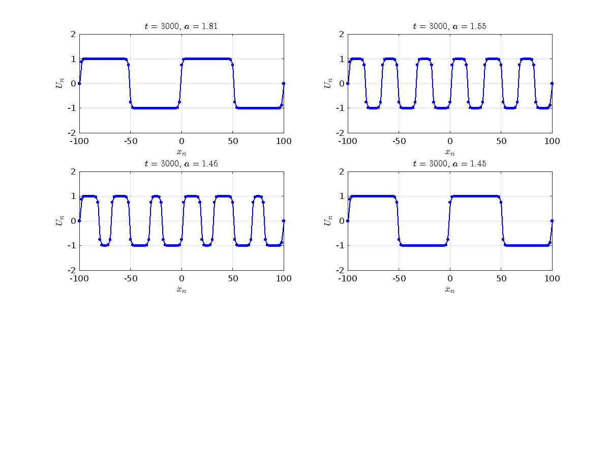
Characteristics for  , with corresponding norm
  where the dynamics appear in the first image of the third row, we observe convergence to a non-linear equilibrium point of branch
  This has the same norm and the same energy as the previous case but the final state has a completely different profile. This result suggests secondary bifurcations have occurred in branch
where the dynamics appear in the first image of the third row, we observe convergence to a non-linear equilibrium point of branch By further reducing the amplitude, distinct values of  are discerned: 1.9, 1.85, 1.81 for which the initial condition
  with norms
  respectively, converges to a non-linear equilibrium point of branch
  This equilibrium point has norm
  and energy
  . The behavior of this equilibrium is illustrated in the third row and in the first image of the third row of Figure 1, and also in the first image of the third row of Figure 2. For all the values between the aforementioned a, the initial condition
  converges to geometrically different non-linear states of branch
  as shown in the second image of the first row and the first image of the second row of Figure 2, for amplitudes
  and
and  respectively.
respectively, converges to a non-linear equilibrium point of branch and energy Refference:
The stationary solutions of the Klein-Gordon equation refer to solutions that are time-independent, meaning they remain constant over time. For the non-linear Klein-Gordon equation you are discussing:
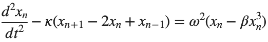
Stationary solutions arise when the time derivative term,  , is zero, meaning the motion of the system does not change over time. This leads to a static differential equation:
, is zero, meaning the motion of the system does not change over time. This leads to a static differential equation:This equation describes how particles in the lattice interact with each other and how non-linearity affects the steady state of the system.
The solutions to this equation correspond to the various possible stable equilibrium states of the system, where each represents different static distribution patterns of displacements  . The specific form of these stationary solutions depends on the system parameters, such as κ , ω, and β , as well as the initial and boundary conditions of the problem.
To find these solutions in a more specific form, one might need to solve the equation using analytical or numerical methods, considering the different cases that could arise in such a non-linear system.
By interpreting the equation in this way, we can relate the dynamics described by the discrete Klein - Gordon equation to the behavior of DNA molecules within a biological system . This analogy allows us to understand the behavior of DNA in terms of concepts from physics and mathematical modeling .
% Parameters
numBases = 100; % Number of spatial points
omegaD = 0.2; % Common parameter for the equation
% Preallocate the array for the function handles
equations = cell(numBases, 1);
% Initial guess for the solution
initialGuess = 0.01 * ones(numBases, 1);
% Parameter sets for kappa and beta
paramSets = [0.1, 0.05; 0.5, 0.05; 0.1, 0.2];
% Prepare figure for subplot
figure;
set(gcf, 'Position', [100, 100, 1200, 400]); % Set figure size
% Newton-Raphson method parameters
maxIterations = 1000;
tolerance = 1e-10;
% Set options for fsolve to use the 'levenberg-marquardt' algorithm
options = optimoptions('fsolve', 'Algorithm', 'levenberg-marquardt', 'MaxIterations', maxIterations, 'FunctionTolerance', tolerance);
for i = 1:size(paramSets, 1)
kappa = paramSets(i, 1);
beta = paramSets(i, 2);
% Define the equations using a function
for n = 2:numBases-1
equations{n} = @(x) -kappa * (x(n+1) - 2 * x(n) + x(n-1)) - omegaD^2 * (x(n) - beta * x(n)^3);
end
% Boundary conditions with specified fixed values
someFixedValue1 = 10; % Replace with actual value if needed
someFixedValue2 = 10; % Replace with actual value if needed
equations{1} = @(x) x(1) - someFixedValue1;
equations{numBases} = @(x) x(numBases) - someFixedValue2;
% Combine all equations into a single function
F = @(x) cell2mat(cellfun(@(f) f(x), equations, 'UniformOutput', false));
% Solve the system of equations using fsolve with the specified options
x_solution = fsolve(F, initialGuess, options);
norm(F(x_solution))
% Plot the solution in a subplot
subplot(1, 3, i);
plot(x_solution, 'o-', 'LineWidth', 2);
grid on;
xlabel('n', 'FontSize', 12);
ylabel('x[n]', 'FontSize', 12);
title(sprintf('\\kappa = %.2f, \\beta = %.2f', kappa, beta), 'FontSize', 14);
end
% Improve overall aesthetics
sgtitle('Stationary States for Different \kappa and \beta Values', 'FontSize', 16); % Super title for the figure
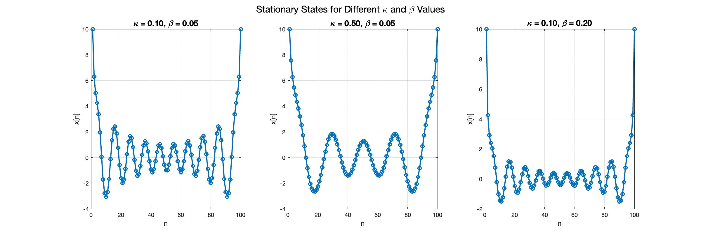
In the second plot, the elasticity constant κis increased to 0.5, representing a system with greater stiffness . This parameter influences how resistant the system is to deformation, implying that a higher κ makes the system more resilient to changes . By increasing κ, we are essentially tightening the interactions between adjacent units in the model, which could represent, for instance, stronger bonding forces in a physical or biological system .
In the third plot the nonlinearity coefficient β is increased to 0.2 . This adjustment enhances the nonlinear interactions within the system, which can lead to more complex dynamic behaviors, especially in systems exhibiting bifurcations or chaos under certain conditions .
This study explores the demographic patterns and disease outcomes during the cholera outbreak in London in 1849. Utilizing historical records and scholarly accounts, the research investigates the impact of the outbreak on the city' s population. While specific data for the 1849 cholera outbreak is limited, trends from similar 19th - century outbreaks suggest a high infection rate, potentially ranging from 30% to 50% of the population, owing to poor sanitation and overcrowded living conditions . Additionally, the birth rate in London during this period was estimated at 0.037 births per person per year . Although the exact reproduction number (R₀) for cholera in 1849 remains elusive, historical evidence implies a high R₀ due to the prevalent unsanitary conditions . This study sheds light on the challenges of estimating disease parameters from historical data, emphasizing the critical role of sanitation and public health measures in mitigating the impact of infectious diseases.
Introduction
The cholera outbreak of 1849 was a significant event in the history of cholera, a deadly waterborne disease caused by the bacterium Vibrio cholera. Cholera had several major outbreaks during the 19th century, and the one in 1849 was particularly devastating.
During this outbreak, cholera spread rapidly across Europe, including countries like England, France, and Germany . The disease also affected North America, with outbreaks reported in cities like New York and Montreal. The exact number of casualties from the 1849 cholera outbreak is difficult to determine due to limited record - keeping at that time. However, it is estimated that tens of thousands of people died as a result of the disease during this outbreak.
Cholera is highly contagious and spreads through contaminated water and food . The lack of proper sanitation and hygiene practices in the 19th century contributed to the rapid spread of the disease. It wasn't until the late 19th and early 20th centuries that advancements in public health, sanitation, and clean drinking water significantly reduced the incidence and impact of cholera outbreaks in many parts of the world.
Infection Rate
Based on general patterns observed in 19th - century cholera outbreaks and the conditions of that time, it' s reasonable to assume that the infection rate was quite high. During major cholera outbreaks in densely populated and unsanitary areas, infection rates could be as high as 30 - 50% or even more.
This means that in a densely populated city like London, with an estimated population of around 2.3 million in 1849, tens of thousands of people could have been infected during the outbreak. It' s important to emphasize that this is a rough estimation based on historical patterns and not specific to the 1849 outbreak. The actual infection rate could have varied widely based on the local conditions, public health measures in place, and the effectiveness of efforts to contain the disease.
For precise and localized estimations, detailed historical records specific to the 1849 cholera outbreak in a particular city or region would be required, and such data might not be readily available due to the limitations of historical documentation from that time period
Mortality Rate
It' s challenging to provide an exact death rate for the 1849 cholera outbreak because of the limited and often unreliable historical records from that time period. However, it is widely acknowledged that the death rate was significant, with tens of thousands of people dying as a result of the disease during this outbreak.
Cholera has historically been known for its high mortality rate, particularly in areas with poor sanitation and limited access to clean water. During cholera outbreaks in the 19th century, mortality rates could be extremely high, sometimes reaching 50% or more in affected communities. This high mortality rate was due to the rapid onset of severe dehydration and electrolyte imbalance caused by the cholera toxin, leading to death if not promptly treated.
Studies and historical accounts from various cholera outbreaks suggest that the R₀ for cholera can range from 1.5 to 2.5 or even higher in conditions where sanitation is inadequate and clean water is scarce. This means that one person with cholera could potentially infect 1.5 to 2.5 or more other people in such settings.
Unfortunately, there are no specific and reliable data available regarding the recovery rates from the 1849 cholera outbreak, as detailed and accurate record - keeping during that time period was limited. Cholera outbreaks in the 19th century were often devastating due to the lack of effective medical treatments and poor sanitation conditions. Recovery from cholera largely depended on the individual's ability to rehydrate, which was difficult given the rapid loss of fluids through severe diarrhea and vomiting .
LONDON CASE OF STUDY
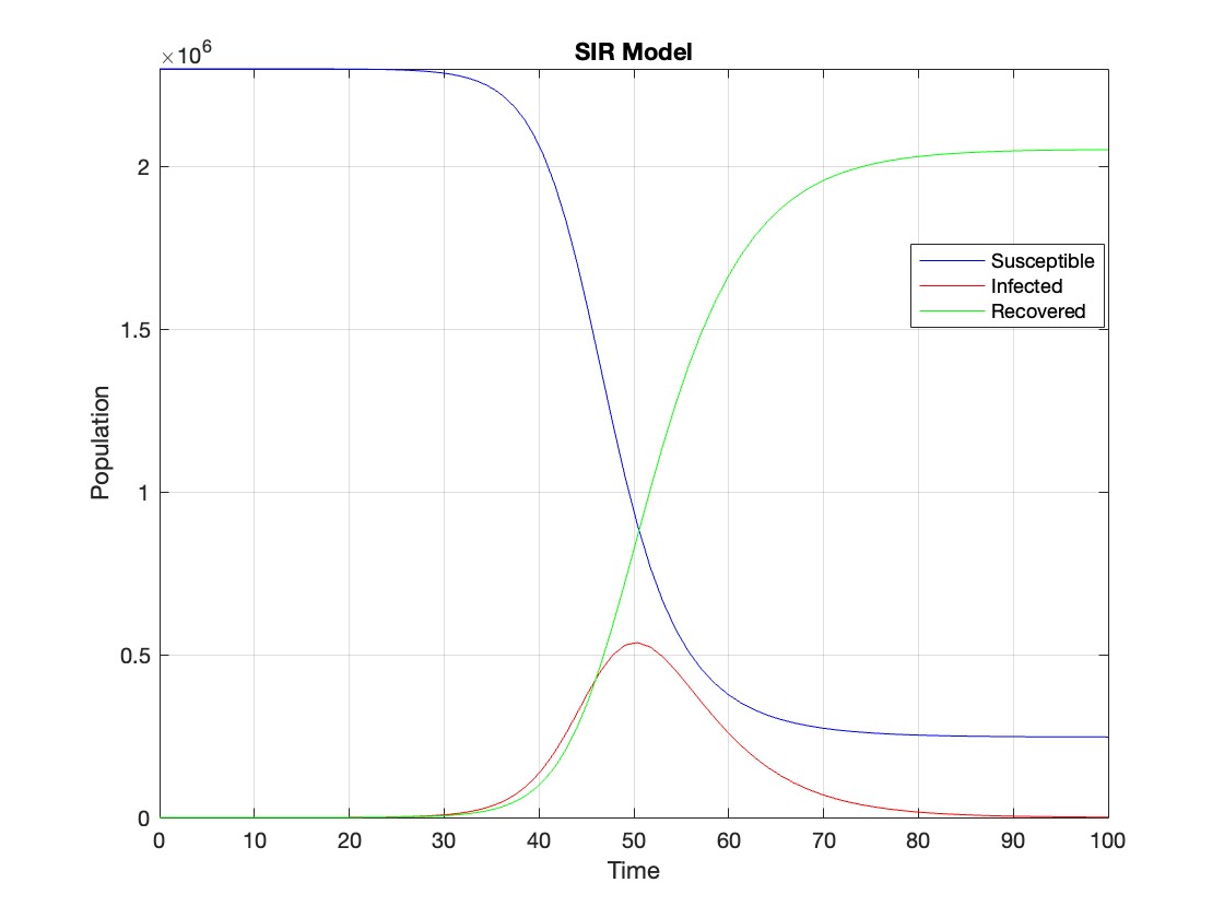
In 1849, the estimated population of London was around 2.3 million people. London experienced significant population growth during the 19th century due to urbanization and industrialization. It’s important to note that historical population figures are often estimates, as comprehensive and accurate record-keeping methods were not as advanced as they are today.
% Define parameters
R0 = 2.5;
beta = 0.5;
gamma = 0.2; % Recovery rate
N = 2300000; % Total population
I0 = 1; % Initial number of infected individuals
% Define the SIR model differential equations
sir_eqns = @(t, Y) [-beta * Y(1) * Y(2) / N; % dS/dt
beta * Y(1) * Y(2) / N - gamma * Y(2); % dI/dt
gamma * Y(2)]; % dR/dt
% Initial conditions
Y0 = [N - I0; I0; 0]; % Initial conditions for S, I, R
% Time span
tmax1 = 100; % Define the maximum time (adjust as needed)
tspan = [0 tmax1];
% Solve the SIR model differential equations
[t, Y] = ode45(sir_eqns, tspan, Y0);
% Plot the results
figure;
plot(t, Y(:,1), 'b', t, Y(:,2), 'r', t, Y(:,3), 'g');
legend('Susceptible', 'Infected', 'Recovered');
xlabel('Time');
ylabel('Population');
title('SIR Model');
axis tight;
grid on;
% Assuming t and Y are obtained from the ode45 solver for the SIR model
% Extract the infected population data (second column of Y)
infected = Y(:,2);
% Plot the infected population over time
figure;
plot(t, infected, 'r');
legend('Infected');
xlabel('Time');
ylabel('Population');
title('Infected Population over Time');
grid on;
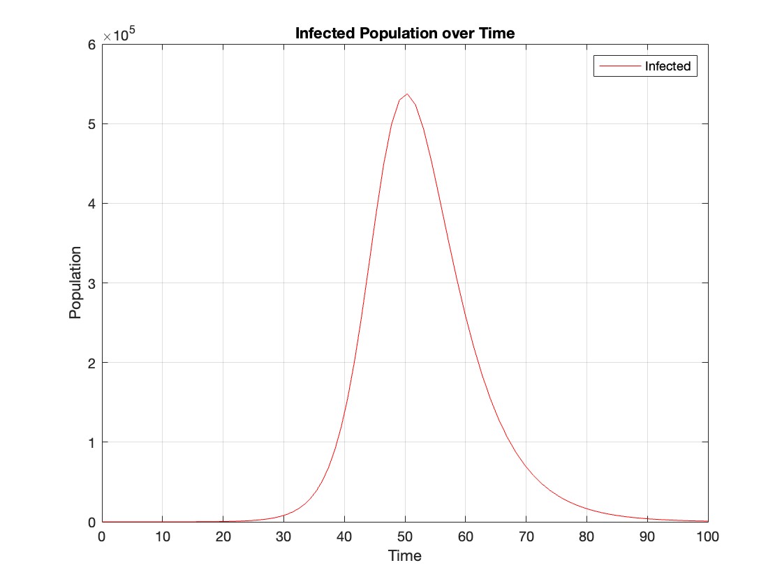
The code provides a visual representation of how the disease spreads and eventually diminishes within the population over the specified time interval . It can be used to understand the impact of different parameters (such as infection and recovery rates) on the progression of the outbreak .
The study of nonlinear dynamical systems in lattices is an area of research with continuously growing interest.The first systematic studies of these systems emerged in the late 1930 s,thanks to the work of Frenkel and Kontorova on crystal dislocations.These studies led to the formulation of the discrete Klein-Gordon equation (DKG).Specifically,in 1939,Frenkel and Kontorova proposed a model that describes the structure and dynamics of a crystal lattice in a dislocation core.The FK model has become one of the fundamental models in physics,as it has been proven to reliably describe significant phenomena observed in discrete media.The equation we will examine is a variation of the following form:

The process described involves approximating a nonlinear differential equation through the Taylor method and simplifying it into a linear model.Let's analyze step by step the process from the initial equation to its final form.For small angles, can be approximated through the Taylor series as:
We substitute  in the original equation with the Taylor approximation:
To map this equation to a linear model,we consider the angles  to correspond to displacements
  in a mass-spring system.Thus,the equation transforms into:
to correspond to displacements We recognize that the term  expresses the nonlinearity of the system,while β is a coefficient corresponding to this nonlinearity,simplifying the expression.The final form of the equation is:
The exact value of β depends on the mapping of coefficients in the Taylor approximation and its application to the specific physical problem.Our main goal is to derive results regarding stability and convergence in nonlinear lattices under nonlinear conditions.We will examine the basic characteristics of the discrete Klein-Gordon equation:
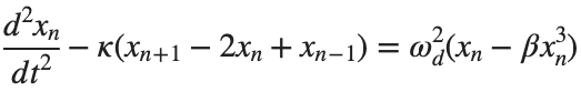
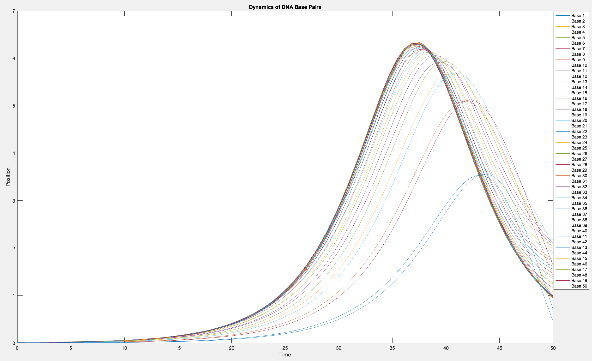
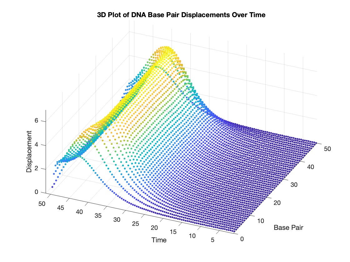
This model is often used to describe the opening of the DNA double helix during processes such as transcription.The model focuses on the transverse motion of the base pairs,which can be represented by a set of coupled nonlinear differential equations.
% Parameters
numBases = 50; % Number of base pairs
kappa = 0.1; % Elasticity constant
omegaD = 0.2; % Frequency term
beta = 0.05; % Nonlinearity coefficient
% Initial conditions
initialPositions = 0.01 + (0.02 - 0.01) * rand(numBases, 1);
initialVelocities = zeros(numBases, 1);
Time span
tSpan = [0 50];
>> % Differential equations
odeFunc = @(t, y) [y(numBases+1:end); ... % velocities
kappa * ([y(2); y(3:numBases); 0] - 2 * y(1:numBases) + [0; y(1:numBases-1)]) + ...
omegaD^2 * (y(1:numBases) - beta * y(1:numBases).^3)]; % accelerations
% Solve the system
[T, Y] = ode45(odeFunc, tSpan, [initialPositions; initialVelocities]);
% Visualization
plot(T, Y(:, 1:numBases))
legend(arrayfun(@(n) sprintf('Base %d', n), 1:numBases, 'UniformOutput', false))
xlabel('Time')
ylabel('Position')
title('Dynamics of DNA Base Pairs')
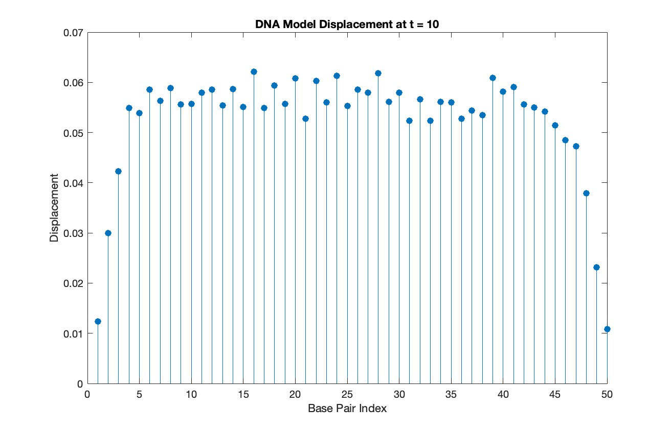
% Choose a specific time for the snapshot
snapshotTime = 10;
% Find the index in T that is closest to the snapshot time
[~, snapshotIndex] = min(abs(T - snapshotTime));
% Extract the solution at the snapshot time
snapshotSolution = Y(snapshotIndex, 1:numBases);
% Generate discrete plot for the DNA model at the snapshot time
figure;
stem(1:numBases, snapshotSolution, 'filled')
title(sprintf('DNA Model Displacement at t = %d', snapshotTime))
xlabel('Base Pair Index')
ylabel('Displacement')
% Time vector for detailed sampling
tDetailed = 0:0.5:50;
% Initialize an empty array to hold the data
data = [];
% Generate the data for 3D plotting
for i = 1:numBases
% Interpolate to get detailed solution data for each base pair
detailedSolution = interp1(T, Y(:, i), tDetailed);
% Concatenate the current base pair's data to the main data array
data = [data; repmat(i, length(tDetailed), 1), tDetailed', detailedSolution'];
end
% 3D Plot
figure;
scatter3(data(:,1), data(:,2), data(:,3), 10, data(:,3), 'filled')
xlabel('Base Pair')
ylabel('Time')
zlabel('Displacement')
title('3D Plot of DNA Base Pair Displacements Over Time')
colormap('rainbow')
colorbar
Hi Guys
Posting this based on a thought I had, so I don't really ahve any code however I would like to know if the thought process is correct and/or relatively accurate.
Consider a simple spring mass system which only allows compression on the spring however when there is tension the mass should move without the effect of the spring distrupting it, thus the mass is just thrown vertically upwards.
The idea which I came up with for such a system is to have two sets of dfferential equations, one which represents the spring system and another which presents a mass in motion without the effects of the spring.
Please refer to the below basic outline of the code which I am proposing. I believe that this may produce relatively decent results. The code essentially checks if there is tension in the system if there is it then takes the last values from the spring mass differential equation and uses it as initial conditions for the differential equation with the mass moving wothout the effects of the spring, this process works in reverse also. The error which would exist is that the initial conditions applied to the system would include effects of the spring. Would there be a better way to code such behaviour?
function xp = statespace(t,x,f,c,k,m)
if (k*x(1)) positive #implying tension
**Use last time step as initial conditions**
**differential equation of a mass moving""
end
if x(1) negative #implying that the mass in now moving down therefore compression in spring
**Use last time step as initial conditions**
**differential equation for a spring mass system**
end
end
The way we've solved ODEs in MATLAB has been relatively unchanged at the user-level for decades. Indeed, I consider ode45 to be as iconic as backslash! There have been a few new solvers in recent years -- ode78 and ode89 for example -- and various things have gotten much faster but if you learned how to solve ODEs in MATLAB in 1997 then your knowledge is still applicable today.
In R2023b, there's a completely new framework for solving ODEs and I love it! You might argue that I'm contractually obliged to love it since I'm a MathWorker but I can assure you this is the real thing!
I wrote it up in a tutorial style on The MATLAB Blog https://blogs.mathworks.com/matlab/2023/10/03/the-new-solution-framework-for-ordinary-differential-equations-odes-in-matlab-r2023b/
The new interface makes a lot of things a much easier to do. Its also setting us up for a future where we'll be able to do some very cool algorithmic stuff behind the scenes.
Let me know what you think of the new functionality and what you think MathWorks should be doing next in the area of ODEs.