Building and Processing a Radar Data Cube
By Rick Gentile and Mike Donovan, MathWorks
The radar data cube provides an intuitive way to represent radar processing as a function of space and time.
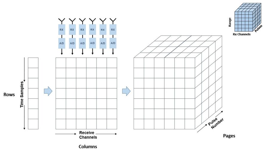
Often referenced in journal papers to demonstrate new algorithms, the radar data cube is a three-dimensional block with the radar returns of a single pulse represented along one axis, returns from additional receiver elements along the second axis, and a collection of the returns from multiple pulses along the third (Figure 1).
Despite this simple construction, engineers may find that developing software to construct and process a radar data cube requires considerable effort. To build a solution in-house, organizations must commit time and resources to write, debug, test, and maintain the necessary code. Challenges exist at each step of the process, including setting up each subsystem of a radar system, modeling complex antenna arrays, simulating propagation through channel models, developing a range of signal processing algorithms, and visualizing the results of system simulations.
MATLAB®, Simulink®, and Phased Array System Toolbox™ process data using the same vector and matrix constructs as those required to build and process radar data cubes. As a result, implementing software to set up a radar data cube, process it, and visualize results requires much less effort and far fewer lines of code in MATLAB than in lower-level programming languages.
This article describes how MATLAB and Phased Array System Toolbox simplify the process of building and processing radar data cubes. Using examples of varying complexity, it outlines the steps needed to build a radar data cube in MATLAB and how to apply beamforming, matched filtering, and Doppler processing with Phased Array System Toolbox to determine the range and speed of a moving object.
The MATLAB code used in this article is available for download.
Building a Radar Data Cube
We begin by modeling the radar system. In this example we will model two systems: an eight-element uniform linear array with a single radar target, and an array with 121 elements mounted on the surface of a sphere and 20 targets.
Modeling an Eight-Element Array and a Single Target
We use Phased Array System Toolbox System objects to model the eight-element uniform linear transmit and receive array. Each element feeds an individual receive channel. The collection of channels makes up the rows of the radar data cube. Spatially sampling the received signals like this enables us to determine the bearing of the target when we use beamforming and direction-of-arrival (DOA) estimation techniques.
We set the radar to transmit and receive multiple pulses at the boresight angle at a pulse repetition interval (PRI) of 1 msec. We then establish a time basis for a collection of pulses that can be expressed in terms of multiple PRIs. This time basis is used to process a set of pulses, which, in turn, provides a basis for evaluating the motion of the target.
To model and simulate this system in MATLAB, we use a set of Phased Array System Toolbox System objects to:
- Initialize a single radar target at a distance of 30 km from the radar with a velocity of 150 m/s
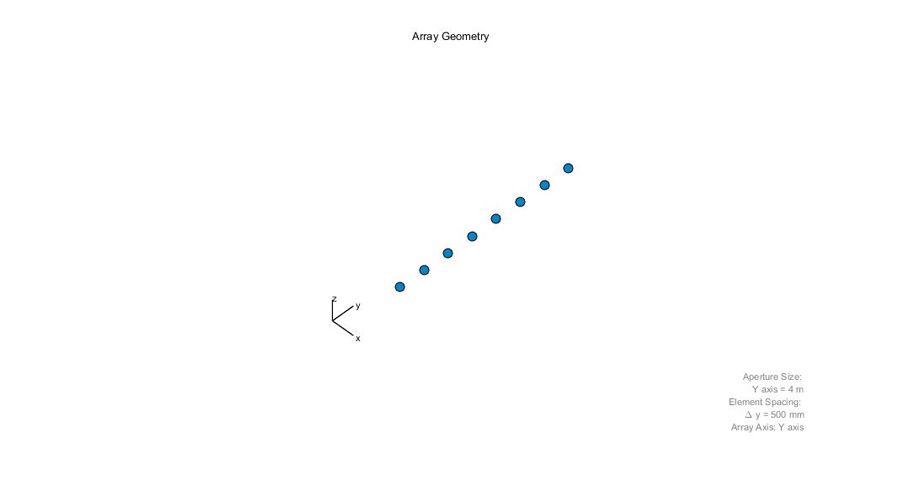
- Create an eight-element array transmitter/receiver (Figure 2)
- Generate a linear FM pulse waveform with a sample rate of 1 MHz and PRF of 1 KHz
- Describe the free space path loss of the propagation channel
- Build the signal processing algorithms
The following code is used to set up the ULA and visualize the array:
% ULA Specs : 8 Element Uniform Linear Array with Cosine Antenna Element
antenna=phased.ULA;
antenna.NumElements = 8;
cosineElement = phased.CosineAntennaElement;
antenna.Element = cosineElement;

viewArray(antenna);
pattern(antenna,300e6,-180:180,0,...
    'Type','directivity',...
    'PropagationSpeed',3e8)
The code to set up the waveform is straightforward and concise:
% Waveform Specs
waveform=phased.LinearFMWaveform;
waveform.SampleRate = 1e6;                     % 1 MHz sample rate
waveform.PRF=1000;                             % Pulse Repetition Frequency of 1000
waveform.PulseWidth=1e-4;                      pulses per second
nSamples = waveform.SampleRate/waveform.PRF;   % Define pulses on 1000 samples
y = step(waveform);
t = (0:nSamples-1)/waveform.SampleRate;
The code to set up the other system components used in the example is similarly concise, and each component contains all parameters needed to fully describe the section of the radar they represent.
Note: Phased Array System Toolbox System represents radar components with System objects. These objects are preceded by a phased prefix in the object name.
The following loop generates the radar pulse, updates the target position, and propagates the pulse to the target and then back to the radar. All returned signals are collected using a receiver array, and the radar data cube is built up pulse by pulse in the loop. The step methods are used to generate or process the data for each component of the radar data cube.
%% Generate radar pulses for ii=1:nPulses wf=step(waveform); [tgtPos, tgtVel] = step(PlatformModel,1/prf); [~, tgtAng] = rangeangle(tgtPos, radarPos); s0 = step(TX, wf); s1 = step(txArray,s0, tgtAng); s2 = step(ChannelModel, s1, radarPos, tgtPos, radarVel, tgtVel); s3 = step(TgtModel, s2); s4 = step(rxArray,s3,tgtAng); s5 = step(rxPreamp,s4); datacube(:,:,ii) = s5(:,:); end |
% Generate waveform % Update target position % Calculate range/angle to target % Amplify signal % Radiate the signal from the array % Propagate from radar to target and return % Reflect signal from Target % Receive the signal at the array % Add rx noise % Build data cube 1 pulse at a time |
In the ChannelModel object we set the parameters to include effects of the roundtrip propagation path. We use the rangeangle function to ensure that we focus the simulation on the regions we are interested in. This helps manage the amount of data being processed and speeds up the simulation.
The radar data cube consists of the complex IQ data samples that are collected at the array for each pulse. The dimensions are 1000 time samples, by 8 receive elements, by 32 pulses (the number of pulses in our coherent processing interval for this example).
Modeling a 121-Element Array and 20 Targets
Our second model is more sophisticated. Instead of one target, we have 20 targets with random positions, velocities, and radar cross section (RCS) values. The following MATLAB code initializes these targets:
%% Simulate with 20 targets and 121 element array
nTgt = 20;          % 20 targets with random postions, velocities and sizes

% Generate random positions, velocities and RCS values
tgtPos=[15e3+abs(randn(1,nTgt))*30e3; abs(randn(1,nTgt))*30e3;zeros(1,nTgt)];
tgtVel=[abs(randn(1,nTgt))*10e2;abs(randn(1,nTgt))*10e2;zeros(1,nTgt)];
RCS = abs(randn(20, 1))';

TgtModel = phased.RadarTarget('MeanRCS',RCS);
Platform = phased.Platform('InitialPosition',tgtPos,'Velocity',tgtVel);
The resulting target-related vectors can be used directly by System objects for position, velocity, and RCS values.
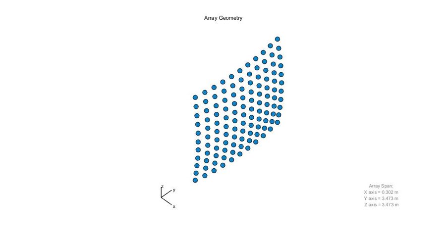
In this example, we increase the bandwidth of the waveform from 1 MHz to 20 MHz (to provide greater resolution) and extend the array to 121 elements mounted on the surface of a sphere. After specifying element positions and norms, we use the phased.ConformalArray object to quickly generate and visualize the array geometry (Figure 3).
antenna = phased.ConformalArray('ElementPosition',ele_pos,   'ElementNormal',ele_normal);
viewArray(antenna)
The initialization code (not shown) requires a few more lines than the previous example to set up the targets and the array. The loop used to build the data cube is identical to the one in the previous example. The only change we made was to use vectors for tgtPos and tgtVel. tgtModel takes in a vector of 20 RCS values.
The dimensions of this cube are 20000 time samples, by 121 receive elements, by 32 pulses. The antenna is much more complex in this example which increases the dimensions by a large factor. Additionally, there are many more targets present. Nevertheless, the code to run the simulation is only incrementally larger.
Processing a Radar Data Cube
With radar data cubes in place, we now apply three array processing algorithms:
- Beamforming
- Matched filtering
- Doppler processing
Beamforming
Beamforming is the process of combining individual receive channels into a single receive signal. It can be helpful to think of beamforming as a spatial filter that applies different complex weights to each of the channels to constructively add signals to be received and destructively add signals to be eliminated. Beamforming works across the rows of the radar data cube, and gives information about the bearing and elevation of the object being tracked.
Beamforming enables us to focus on a specific region in space to improve the signal-to-noise ratio of our detections. It also has the benefit of de-emphasizing noise and interference from areas outside the area of interest.
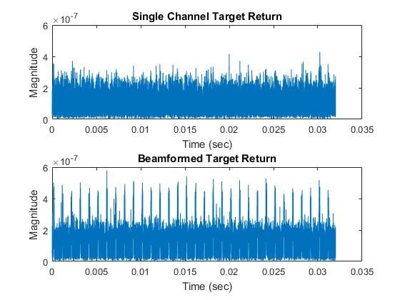
Using the first example as the basis for the processing, we plot the original return for a single channel together with the beamformed target return and it is easy to see the difference. The target clearly becomes visible when beamforming is used (Figure 4).
To create a phase shift beamformer with Phased Array System Toolbox we first establish the PhaseShiftBeamformer object and associate it with the eight-element ULA antenna we modeled earlier. We also enable the input port to provide a direction to form our beam.
%% Peform beamforming
% Beamformer Specs
beamformer=phased.PhaseShiftBeamformer;
beamformer.SensorArray=antenna;
beamformer.DirectionSource='Input port';
beamformer.WeightsOutputPort=true;
beamformer.WeightsNormalization='Preserve power';


[bf0,w0]=step(beamformer,datacube(:,:,1),[0;0]);
[bf, w]=step(beamformer,datacube(:,:,1),[30;0]);
For illustration purposes, we used two separate calls to the step method. The first steers the beam to a zero degree azimuth (broadside from the array). The second steers it to a 30 degree azimuth where the moving object is actually located. In this example, the target locations were fixed for simplicity. In a full-featured system, additional System objects would be used to determine a direction of arrival and feed an azimuth and elevation angle to the beamformer directly.
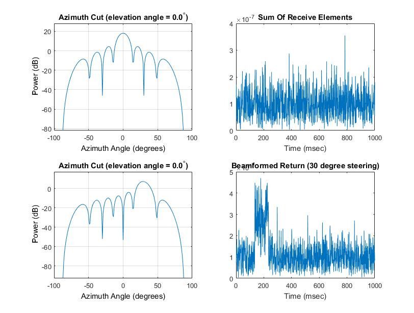
To visualize the results, we plot the response of the ULA, the sum of the receive elements, and the beamformed return (Figure 5). With no beamforming, the peak of the pattern response is at zero degrees azimuth, which is the boresight angle with no steering. Most of the beam formed from the receive array is concentrated on an area where the target is not located. In addition, one of the nulls is at 30 degrees off boresight, where the target is located.
However, when we use phased array weights and the beamformer to steer the array to a 30- degree azimuth, we produce an enhanced target return where we can easily see the target return distinguished from the noise.
Matched Filtering
The matched filtering algorithm applies pulse compression to the return signal, a technique that enables systems to transmit a longer pulse width without sacrificing resolution. Performed on the data that makes up the columns of the radar data cube, matched filtering enhances the radar return by correlating the receive time samples with a sampled version of the source waveform.
To implement matched filtering in MATLAB, we use the getmatchedfilter function to return the matched filter coefficients that correspond to the transmit waveform and use the phased.MatchedFilter System object to process the time samples for the radar pulse return.
%% Perform matched filtering
b = getMatchedFilter(waveform);

matchedfilter = phased.MatchedFilter(...
    'Coefficients',b,...
	'SpectrumWindow','Hamming');

matchFiltered = step(matchedfilter,beamformed);
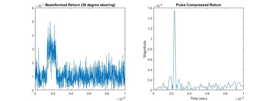
The result of performing a matched filter on the beamformed return is a sharp peak at the range bin of the moving object (Figure 6). One advantage of using a modulated pulse (as we have done with the linear FM waveform) is that the correlated pulse produces a narrow peak at the target return. Once we detect this peak, we can calculate the distance to the moving object. The index of the time sample where the peak exists tells us the distance to the object.
In this case, we use the time2range function to account for the length of the matched filter when we convert the time to distance. For this example, the calculated distance is 19.94 km.
Doppler Processing
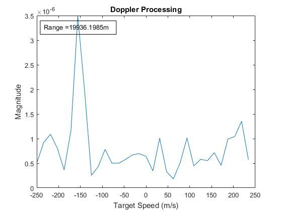
To determine the speed of the target, we use the Doppler shift observed in the target returns. In this case, we compute the fast Fourier transform across all pulses (or pages) in the range bin where the target is located. We can see the peak at a frequency that corresponds to a radial velocity of 150m/s (Figure 7).
This Doppler resolution depends on the number of pulses in the coherent processing interval. As a result, we can improve the accuracy of the speed measurement, by sending more pulses at this target.
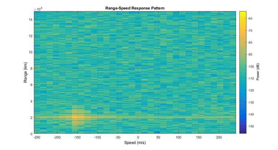
We compute the range Doppler pattern using Phased Array System Toolbox and plot the results (Figure 8).
Extending the Examples
Now that we have the MATLAB code to build a radar data cube and process it using beamforming to estimate the range and Doppler of a moving object, we are well positioned to make improvements. We could, for example extend the code to extract even more information about the target returns contained in the radar data cube using DOA estimation, angle-Doppler response plots, space-time adaptive processing (STAP), and other algorithms available through Phased Array System Toolbox.
Published 2016 - 92958v00
