Main Content

initial

System response to initial states of state-space model

    Description

    For state-space and sparse state-space models, initial computes the unforced system response y to initial states x0.

    • Continuous time:

      x˙=Ax,x(t0)=x0y=Cx

    • Discrete time:

      x[k+1]=Ax[k]x[k0]=x0y=Cx[k]

    For linear time-varying or linear parameter-varying state-space models, initial computes the response with initial state x0, initial parameter p0 (LPV models), and input held to the offset value (u(t) = u0(t) or u(t) = u0(t,p). This corresponds to the initial condition response of the local linear dynamics.

    Initial Response Plots

    example

    initial(sys,x0) plots the unforced system response to initial states of a state-space (ss) model sys with an initial condition on the states specified by the vector x0:

    The state-space model sys can be continuous-time or discrete-time, and SISO or MIMO. For MIMO state-space systems, the plot displays the responses for the outputs of each channel. initial automatically determines the time steps and duration of the simulation based on the system dynamics.

    example

    initial(sys,x0,tFinal) plots the simulated response from t = 0 to the final time t = tFinal. The function uses system dynamics to determine the intervening time steps.

    example

    initial(sys,x0,t) plots the response at the times that you specify in the vector t.

    initial(sys,x0,t,p) also specifies the parameter trajectory p for lpvss models.

    example

    initial(sys,{x0,p0},t,p) also specifies the initial parameter value p0 and parameter trajectory p for LPV models. p0 is required for implicit parameter trajectories.

    example

    initial(sys1,sys2,...,sysN,x0,___) plots the response of multiple dynamic systems on the same plot. All systems must have the same number of inputs and outputs. You can use multiple dynamic systems with any of the previous input-argument combinations.

    example

    initial(sys1,LineSpec1,...,sysN,LineSpecN,x0,___) specifies a color, line style, and marker for each system in the response plot. You can use LineSpec with any of the previous input-argument combinations. When you need additional plot customization options, use initialplot instead.

    Initial Response Data

    y = initial(sys,x0,t) returns the initial response sys at the times specified in the vector t. This syntax does not draw a plot.

    y = initial(sys,x0,t,p) also specifies the parameter trajectory p for LPV models.

    example

    y = initial(sys,{x0,p0},t,p) also specifies the initial parameter value and parameter trajectory p for LPV models. p0 is required for implicit parameter trajectories.

    example

    [y,tOut,x] = initial(sys,x0) returns the output response y, the time vector tOut and the state trajectories x. The array y has as many rows as time samples (length of tOut) and as many columns as outputs. Similarly, x has length(tOut) rows and as many columns as states.

    [y,tOut,x,pOut] = initial(sys,x0,t,p) also returns parameter trajectories pOut, when sys is an lpvss model.

    Examples

    collapse all

    For this example, generate a random state-space model with 5 states and create the plot for the system response to the initial states.

    rng("default")
    sys = rss(5);
    x0 = [1,2,3,4,5];
    initial(sys,x0)

    Figure contains an axes object. The axes object contains an object of type line. These objects represent Driving inputs, sys.

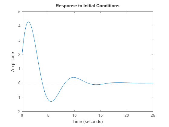
    Plot the response of the following state-space model:

    [x˙1x˙2]=[-0.5572-0.78140.78140][x1x2]y=[1.96916.4493][x1x2].

    Take the following initial condition:

    x(0)=[10].

    a = [-0.5572, -0.7814; 0.7814, 0];
    c = [1.9691  6.4493];
    x0 = [1 ; 0];
    
    sys = ss(a,[],c,[]);
    initial(sys,x0)

    Figure contains an axes object. The axes object contains an object of type line. These objects represent Driving inputs, sys.

    Consider the following two-input, two-output dynamic system.

    sys(s)=[03ss2+s+10s+1s+52s+6].MIMO system

    Convert the sys to state-space form since initial condition response plots are supported only for state-space models.

    sys = ss([0, tf([3 0],[1 1 10]) ; tf([1 1],[1 5]), tf(2,[1 6])]);
    size(sys)
    State-space model with 2 outputs, 2 inputs, and 4 states.
    

    The resultant state-space model has four states. Hence, provide an initial condition vector with four elements.

    x0 = [0.3,0.25,1,4];

    Create the initial condition response plot.

    initial(sys,x0);

    Figure contains 2 axes objects. Axes object 1 with ylabel To: Out(1) contains an object of type line. These objects represent Driving inputs, sys. Axes object 2 with ylabel To: Out(2) contains an object of type line. These objects represent Driving inputs, sys.

    The resultant plot contains two subplots - one for each output in sys.

    For this example, examine the initial condition response of the following zero-pole-gain model and limit the plot to tFinal = 15 s.

    First, convert the zpk model to an ss model since initial only supports state-space models.

    sys = ss(zpk(-1,[-0.2+3j,-0.2-3j],1)*tf([1 1],[1 0.05]));
    tFinal = 15;
    x0 = [4,2,3];

    Now, create the initial conditions response plot.

    initial(sys,x0,tFinal);

    Figure contains an axes object. The axes object contains an object of type line. These objects represent Driving inputs, sys.

    For this example, plot the initial condition responses of three dynamic systems.

    First, create the three models and provide the initial conditions. All the models should have the same number of states.

    rng('default');
    sys1 = rss(4); 
    sys2 = rss(4);
    sys3 = rss(4);
    x0 = [1,1,1,1];

    Plot the initial condition responses of the three models using time vector t that spans 5 seconds.

    t = 0:0.1:5;
    initial(sys1,'r--',sys2,'b',sys3,'g-.',x0,t)

    Figure contains an axes object. The axes object contains 3 objects of type line. These objects represent Driving inputs, sys1, sys2, sys3.

    Extract the initial condition response data of the following state-space model with two states:

    [x˙1x˙2]=[-0.5572-0.78140.78140][x1x2]y=[1.96916.4493][x1x2].

    Use the following initial conditions:

    x(0)=[10].

    a = [-0.5572, -0.7814; 0.7814, 0];
    c = [1.9691  6.4493];
    x0 = [1 ; 0];
    sys = ss(a,[],c,[]);
    [y,tOut,x] = initial(sys,x0);

    The array y has as many rows as time samples (length of tOut) and as many columns as outputs. Similarly, x has rows equal to the number of time samples (length of tOut) and as many columns as states.

    For this example, extract the initial condition response data of a state-space model with 6 states, 3 outputs and 2 inputs.

    First, create the model and provide the initial conditions.

    rng('default');
    sys = rss(6,3,2); 
    x0 = [0.1,0.3,0.05,0.4,0.75,1];

    Extract the initial condition responses of the model using time vector t that spans 15 seconds.

    t = 0:0.1:15;
    [y,tOut,x] = initial(sys,x0,t);

    The array y has as many rows as time samples (length of tOut) and as many columns as outputs. Similarly, x has rows equal to the number of time samples (length of tOut) and as many columns as states.

    For this example, consider lpvHCModel.m that defines the following model.

    x˙=-(x-x0(p))+(u-u0(p))

    y=y0(p)+(1-p2)(x-x0(p))

    (x0(p),u0(p),y0(p))=(tanh-1(p),tanh-1(p),p)

    Use lpvss to construct this LPV plant. Since tanh-1(p) is infinite for |p|=1, clip p to the range [-pmax,pmax] to stay away from singularity.

    pmax = 0.99;
    vSys = lpvss('p',@(t,p) lpvHCModel(t,p,pmax),'StateName','x');

    You can compute the initial response for this model along a trajectory p(t).

    Define p(t) implicitly as a function F(t,x,u) of time t, state x, and input u. For this model, use p(t)=y(t)=tanh(x).

    pinit = 0.5;
    xinit = 0.5;
    t= linspace(0,1,100);
    p = @(t,x,u) tanh(x);
    initial(vSys,{xinit,pinit},t,p);

    Figure contains an axes object. The axes object contains an object of type line. These objects represent Driving inputs, vSys.

    initial computes the response with initial state, initial parameter, and input held to offset value u0(t,p).

    Input Arguments

    collapse all

    Dynamic system, specified as a SISO or MIMO dynamic system model or array of dynamic system models. You can only use state-space models of the following types:

    • Continuous-time or discrete-time numeric ss models.

    • Generalized or uncertain LTI models such as genss or uss models. (Using uncertain models requires Robust Control Toolbox™ software.)

      • For tunable control design blocks, the function evaluates the model at its current value for both plotting and returning response data.

      • For uncertain control design blocks, the function plots the nominal value and random samples of the model. When you use output arguments, the function returns response data for the nominal model only.

    • Sparse state-space models such as sparss and mechss models. You must specify final time tFinal for sparse state-space models.

    • Linear time-varying (ltvss) and linear parameter-varying (lpvss) models.

    If sys is an array of models, the function plots the responses of all models in the array on the same axes.

    End time to compute the response, specified as a positive scalar value. initial simulates the response from t = 0 to t = tFinal.

    • For continuous-time systems, the function determines the step size and number of points automatically from system dynamics. Express tFinal in the system time units, specified in the TimeUnit property of sys.

    • For discrete-time systems, the function uses the sample time of sys as the step size. Express tFinal in the system time units, specified in the TimeUnit property of sys.

    • For discrete-time systems with unspecified sample time (Ts = -1), initial interprets tFinal as the number of sampling periods to simulate.

    Time vector at which to compute the response, specified as a vector of positive scalar values. Express t in the system time units, specified in the TimeUnit property of sys.

    • For continuous-time models, specify t in the form Ti:dt:Tf. To obtain the response at each time step, the function uses dt as the sample time of a discrete approximation to the continuous system.

    • For discrete-time models, specify t in the form Ti:Ts:Tf, where Ts is the sample time of sys.

    Line style, marker, and color, specified as a string or vector of one, two, or three characters. The characters can appear in any order. You do not need to specify all three characteristics (line style, marker, and color). For example, if you omit the line style and specify the marker, then the plot shows only the marker and no line. For more information about configuring this argument, see the LineSpec input argument of the plot function.

    Example: 'r--' specifies a red dashed line

    Example: '*b' specifies blue asterisk markers

    Example: 'y' specifies a yellow line

    Initial condition of the states, specified as a vector. x0 must have the same length as the number of states in sys.

    Parameter trajectory of the LPV model, specified as a matrix or a function handle.

    • For exogenous or explicit trajectories, specify p as a matrix with dimensions N-by-Np, where N is the number of time samples and Np is the number of parameters.

      Thus, the row vector p(i,:) contains the parameter values at the ith time step.

    • For endogenous or implicit trajectories, specify p as a function handle of the form p = F(t,x,u) in continuous time and p = F(k,x,u) in discrete time that gives parameters as a function of time t or time sample k, state x, and input u. The initial parameter value p0 is required for this input method.

    Initial value of the parameters of LPV model, specified as a vector. p0 must have the same length as the number of parameters in sys.

    Output Arguments

    collapse all

    Response data, returned as an array.

    • For SISO systems, y is a column vector of the same length as t (if provided) or tOut (if you do not provide t).

    • For single-input, multi-output systems, y is a matrix with as many rows as there are time samples and as many columns as there are outputs. Thus, the jth column of y, or y(:,j), contains the response of from the input to the jth output.

    • For MIMO systems, the dimensions of y are then N-by-Ny, where:

      • N is the number of time samples.

      • Ny is the number of system outputs.

    Times at which response is computed, returned as a vector. When you do not provide a specific vector t of times, initial chooses this time vector based on the system dynamics. The times are expressed in the time units of sys.

    State trajectories, returned as an array. x contains the evolution of the states of sys at each time in t or tOut. The dimensions of x are N-by-Nx, where:

    • N is the number of time samples.

    • Nx is the number of states.

    Parameter trajectories, returned as an array. When sys is a linear-parameter varying (lpvss) model, pOut contains the evolution of the parameters of sys. The dimensions of pOut are N-by-Np, where:

    • N is the number of time samples.

    • Np is the number of parameters.

    Version History

    Introduced before R2006a