interface
(Not recommended) Specify physical connections between components of
mechss model
interface is not recommended. Use addInterface and
assemble
instead. For more information, see Version History.
Syntax
Description
sysCon = interface(sys,C1,IC1,C2,IC2)C1 and
C2 in the second-order sparse model sys.
IC1 and IC2 contain the indices of the coupled
degrees of freedom (DOFs) relative to the DOFs of C1 and
C2. The physical interface is assumed rigid and satisfies the standard
consistency and equilibrium conditions. sysCon is the resultant model
with the specified physical connections. Use showStateInfo
to get the list of all available components of sys.
sysCon = interface(___,method)method =
'dual' and the function uses the dual-assembly method of physical
coupling. Set method = 'primal' to use the
primal-assembly method of physical coupling. For more information, see Algorithms.
Examples
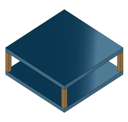
For this example, consider a structural model that consists of two square plates connected with pillars at each vertex as depicted in the figure below. The lower plate is attached rigidly to the ground while the pillars are attached rigidly to each vertex of the square plate.
Load the finite element model matrices contained in
platePillarModel.mat and create the sparse second-order model
representing the above system.
load('platePillarModel.mat')
model = ...
   mechss(M1,[],K1,B1,F1,'Name','Plate1') + ...
   mechss(M2,[],K2,B2,F2,'Name','Plate2') + ...
   mechss(Mp,[],Kp,Bp,Fp,'Name','Pillar3') + ...
   mechss(Mp,[],Kp,Bp,Fp,'Name','Pillar4') + ...
   mechss(Mp,[],Kp,Bp,Fp,'Name','Pillar5') + ...
   mechss(Mp,[],Kp,Bp,Fp,'Name','Pillar6');
sys = model;
Use showStateInfo to examine the components of the
mechss model object.
showStateInfo(sys)
The state groups are:

    Type        Name      Size
  ----------------------------
  Component    Plate1     2646
  Component    Plate2     2646
  Component    Pillar3     132
  Component    Pillar4     132
  Component    Pillar5     132
  Component    Pillar6     132
Now, load the interfaced degree of freedom (DOF) index data from
dofData.mat and use interface to create the
physical connections between the two plates and the four pillars.
dofs is a 6x7 cell array where the first two
rows contain DOF index data for the first and second plates while the remaining four
rows contain index data for the four pillars. By default, the function uses
dual-assembly method of physical coupling.
load('dofData.mat','dofs')
for i=3:6
   sys = interface(sys,"Plate1",dofs{1,i},"Pillar"+i,dofs{i,1});
   sys = interface(sys,"Plate2",dofs{2,i},"Pillar"+i,dofs{i,2});
end
Specify connection between the bottom plate and the ground.
sysConDual = interface(sys,"Plate2",dofs{2,7});Use showStateInfo to confirm the physical interfaces.
showStateInfo(sysConDual)
The state groups are:

    Type            Name         Size
  -----------------------------------
  Component        Plate1        2646
  Component        Plate2        2646
  Component       Pillar3         132
  Component       Pillar4         132
  Component       Pillar5         132
  Component       Pillar6         132
  Interface    Plate1-Pillar3      12
  Interface    Plate2-Pillar3      12
  Interface    Plate1-Pillar4      12
  Interface    Plate2-Pillar4      12
  Interface    Plate1-Pillar5      12
  Interface    Plate2-Pillar5      12
  Interface    Plate1-Pillar6      12
  Interface    Plate2-Pillar6      12
  Interface    Plate2-Ground        6
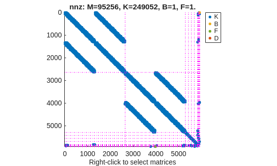
You can use spy to visualize the sparse matrices in the final
model.
spy(sysConDual)
Now, specify physical connections using the primal-assembly method.
sys = model;
for i=3:6
   sys = interface(sys,"Plate1",dofs{1,i},"Pillar"+i,dofs{i,1},'primal');
   sys = interface(sys,"Plate2",dofs{2,i},"Pillar"+i,dofs{i,2},'primal');
end
sysConPrimal = interface(sys,"Plate2",dofs{2,7},'primal');
Use showStateInfo to confirm the physical interfaces.
showStateInfo(sysConPrimal)
The state groups are:

    Type        Name      Size
  ----------------------------
  Component    Plate1     2646
  Component    Plate2     2640
  Component    Pillar3     108
  Component    Pillar4     108
  Component    Pillar5     108
  Component    Pillar6     108
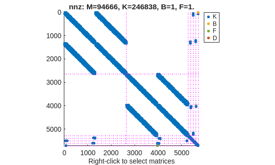
Primal assembly eliminates half of the redundant DOFs associated with the shared set of DOFs in the global finite element mesh.
You can use spy to visualize the sparse matrices in the final
model.
spy(sysConPrimal)
The data set for this example was provided by Victor Dolk from ASML.
Input Arguments
Output Arguments
Algorithms
Version History
Introduced in R2020bSee Also
addInterface | assemble | mechss | xsort | showStateInfo