Power Amplifier Modeling Using Neural Networks

Since R2024a

This example shows how to model a power amplifier (PA) using several different neural network (NN) architectures. In this example, you will

• Design and train different PA neural models.

• Test the different PA networks using an actual PA.

• Compare the results of all the PA networks to that of the actual PA.

Introduction

Power amplifiers lie at the front end of most radio frequency systems, including wireless communications and radar systems, and are critical in ensuring the appropriate range of wireless systems. Power amplifier behavior is affected by nonlinear behavior and memory effects, and hence depends on input signal characteristics such as bandwidth, frequency, PAPR, modulation, and loading conditions. Some popular behavior models include memory polynomial (MP), envelope memory polynomial (EMP), generalized memory polynomial (GMP), and Volterra series (VS).

Recent studies show that neural networks have the potential to more accurately model wideband PAs. This example models, trains, and tests the following neural network architectures:

• Augmented real-valued time-delay neural network power amplifier (ARVTDNNPA)

• Long short-term memory neural network power amplifier (LSTMNNPA)

• Bidirectional LSTM neural network power amplifier (BiLSTMNNPA)

• Gated recurrent unit neural network power amplifier (GRUNNPA)

Following diagram shows the training workflow. During training, measure the input to the PA, $$u$$, used as the input signal and the output of the PA, $$x$$, used as the target signal.

NN-based PA Structure

Design of following types of neural network power amplifier (NN-PA):

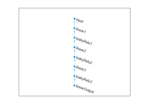
• ARVTDNNPA $-$Has multiple fully connected layers with leakyRelu activation and an augmented input.

• LSTMNNPA$-$Has lstm and fully connected layers with tanh activation and an augmented input.

• BiLSTMNNPA$-$Has bilstm and fully connected layers with tanh activation and an augmented input.

• GRUNNPA$-$Has gru and fully connected layers with tanh activation and an augmented input.

The memory polynomial model has been commonly applied in the behavioral modeling and predistortion of PAs with memory effects. This equation shows the PA memory polynomial.

$\mathit{x}\left(\mathit{n}\right)=\mathit{f}\left(\mathit{u}\left(\mathit{n}\right)\right)=\sum _{\mathit{m}=0}^{\mathit{M}-1}\sum _{\mathit{k}=0}^{\mathit{K}-1}{\mathit{c}}_{\mathit{m}}\mathit{u}\left(\mathit{n}-\mathit{m}\right){\left|\mathit{u}\left(\mathit{n}-\mathit{m}\right)\right|}^{\mathit{k}}$

The output is a function of the delayed versions of the input signal, $$u(n)$$, and also powers of the amplitudes of $$u(n)$$ and its delayed versions. Since a neural network can approximate any function provided that it has enough layers and neurons per layer, you can input $$u(n)$$ to the neural network and approximate $$f(u(n))$$. The neural network can input $$u(n-m)$$ and $$|u(n-m){|}^k$$ to decrease the required complexity.

The input layer inputs the in-phase and quadrature components (${\mathit{I}}_{\mathrm{in}}$/${\mathit{Q}}_{\mathrm{in}}$) of the complex baseband samples. The ${\mathit{I}}_{\mathrm{in}}$/${\mathit{Q}}_{\mathrm{in}}$ samples and $$m$$ delayed versions are used as part of the input to account for the memory in the PA model. Also, the amplitudes of the ${\mathit{I}}_{\mathrm{in}}$/${\mathit{Q}}_{\mathrm{in}}$ samples up to the $$k^{th}$$ power are fed as input to account for the nonlinearity of the PA.

Where,

$$\begin{array}{l}{I}_{in}(n)=\mathrm{\Re }(x(n))\\ Q_{in}(n)=\mathrm{\Im }(x(n))\\ I_{out}(n)=\mathrm{\Re }(u(n))\\ Q_{out}(n)=\mathrm{\Im }(u(n)),\end{array}$$

$$\mathrm{\Re }$$ and $$\mathrm{\Im }$$ are the real and imaginary part operators, respectively.

Power Amplifier Dataset Creation

Data Preparation for Neural Network Digital Predistortion Design (Communications Toolbox) example shows how to prepare training, validation, and testing data. Use the training and validation data to train the NN-PA. Use the test data to evaluate the NN-PA performance.

Choose Data Source

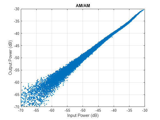
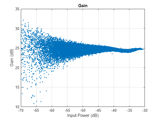
Choose the data source for the system. This example uses an NXP Airfast LDMOS Doherty PA, which is connected to a local NI VST, as described in the Power Amplifier Characterization (Communications Toolbox) example. If you do not have access to a PA, run the example with saved data. If you choose saved data, the example downloads the data files.

dataSource = "Saved data";

Generate Training, Validation and Testing Data

Generate Over-sampled OFDM Signals

Generate OFDM-based signals to excite the PA. This example uses a 5G-like OFDM waveform. Set the bandwidth of the signal to 100 MHz. Choosing a larger bandwidth signal causes the PA to introduce more nonlinear distortion and yields greater benefit from the addition of the DPD. Generate six OFDM symbols, where each subcarrier carries a 16-QAM symbol, by using the helperNNDPDGenerateOFDM function. Save the 16-QAM symbols as a reference to calculate the EVM performance. To capture the effects of higher order nonlinearities, the example oversamples the PA input by a factor of 5.

bw          = 100e6; % Hz
symPerFrame = 6; % OFDM symbols per frame
M           = 16; % Each OFDM subcarrier contains a 16-QAM symbol
osf         = 5; % oversampling factor for PA input
[txWaveTrain, txWaveVal, txWaveTest, ...
    qamRefSymTrain, qamRefSymVal, qamRefSymTest, ...
    ofdmParams] = helperOversampledOFDMSignals(bw, symPerFrame, M, osf);
Fs = ofdmParams.SampleRate;

Pass signals through the PA using the helperVSTDriver and helperNNDPDPAMeasure functions.

switch dataSource
    case "Data acquisition - NI VST"
        resourceName            =  'VST_01';
        VST = helperVSTDriver(resourceName);
        cleanup = onCleanup(@()release(VST));
        VST.DUTExpectedGain     = 29; % dB
        VST.ExternalAttenuation = 30; % dB
        VST.DUTTargetInputPower = 5; % dBm
        VST.CenterFrequency     = 3700000000; % Hz

Send the signals to the PA and collect the outputs

        [paOutputTrain, measInfo] = helperNNDPDPAMeasure(txWaveTrain, Fs, VST);
        linearGainPA = measInfo.LinearGain;
        paOutputVal = helperNNDPDPAMeasure(txWaveVal, Fs, VST);
        paOutputTest = helperNNDPDPAMeasure(txWaveTest, Fs, VST);
    otherwise
        helperNNDPDDownloadData("dataprep")
        load("nndpdTrainingDataOct23.mat", ...
            "txWaveTrain", "qamRefSymTrain", "paOutputTrain", ...
            "txWaveVal", "qamRefSymVal", "paOutputVal", ...
            "txWaveTest", "qamRefSymTest", "paOutputTest", ...
            "linearGainPA");
end

Starting download of data files from:
	https://www.mathworks.com/supportfiles/spc/NNDPD/NNDPD_training_data_Oct23.zip
Download complete. Extracting files.
Extract complete.

helperPANNPlotSpecAnAMAM(txWaveTrain, paOutputTrain);

helperPANNPlotSpecAnGain(txWaveTrain, paOutputTrain, linearGainPA);

Preprocess Data

Enter the memory depth and non-linear degree of power amplifier.

memDepth        = 5;% Memory depth of the PA model
nonlinearDegree = 5; % Nonlinear polynomial degree

Preprocess data to generate input vectors containing features.

paInputTrain = txWaveTrain;
paInputVal = txWaveVal;
paInputTest = txWaveTest;

scalingFactorPA = 1/std(paInputTrain);
inputProcPA = dpdPreprocessor(memDepth, nonlinearDegree);
inputFeaturesTrain = inputProcPA(paInputTrain*scalingFactorPA);
reset(inputProcPA)
inputFeaturesVal = inputProcPA(paInputVal*scalingFactorPA);

paOutputTrainNorm = paOutputTrain*scalingFactorPA;
paOutputTrainR = [real(paOutputTrainNorm) imag(paOutputTrainNorm)];
paOutputValNorm = paOutputVal*scalingFactorPA;
paOutputValR = [real(paOutputValNorm) imag(paOutputValNorm)];

Design and Train

Before training the neural network based PA, select the memory depth and degree of nonlinearity in the Pre-processing Data section. For purposes of comparison, specify a memory depth of 5 and a nonlinear polynomial degree of 5, as in the Power Amplifier Characterization (Communications Toolbox) example.

Define NN-PA

Select one of the NN-PA network architectures.

networkArch          = "ARVTDNNPA"; % Select the power amplifier neural network
enableAnalyzeNetwork = false; % Enable to analyze the NN-PA model using analyzeNetwork
inputLayerDim        = 2*memDepth+(nonlinearDegree-1)*memDepth;
switch networkArch
    case "ARVTDNNPA"
        NNPANet = arvtdnnpaModel(inputLayerDim);
    case "LSTMNNPA"
        NNPANet = lstmnnpaModel(inputLayerDim);
    case "BiLSTMNNPA"
        NNPANet = bilstmnnpaModel(inputLayerDim);
    case "GRUNNPA"
        NNPANet = grunnpaModel(inputLayerDim);
end
NNPANet.plot()

% Analyze the selected NN-PA architecture
if enableAnalyzeNetwork
    NNPANetInfo = analyzeNetwork(NNPANet);
end

Load Network Parameters

Create MatFile object for PANNModels.mat file which contains pre-trained network models and training parameters.

powerAmpModels = helperManagePAModels(true);

Training NN-PA

Set the memory depth and degree of non-linearity to 5 for the power amplifier in the Pre-processing Data section. See the Power Amplifier Characterization (Communications Toolbox) example for more details.

trainNow  = false; % Enable to train the selected network
saveToMAT = true; % Enable to save the trained model or computed performance metrics or both to MAT file

if trainNow
    solverName         = "adam"; % Select the solver for training
    miniBatchSize      = 4096; % Mini-batch size for training
    numEpochs          = 1000; % Number of epochs for training
    exeEnvironment     = "auto"; % Select the execution environment
    lossFcn            = "mse"; % MSE loss function
    enableVerbose      = true; % Enable verbose to see the training progress printed
    trainingPlot       = "none"; % Select "training-progress" to see dynamic plot of training
    numSamples         = size(inputFeaturesVal, 1);
    iterationsPerEpoch = floor(numSamples/miniBatchSize);

    options = trainingOptions(solverName, ...
        MaxEpochs=numEpochs, ...
        MiniBatchSize=miniBatchSize, ...
        InitialLearnRate=2e-2, ...
        LearnRateDropFactor=0.5, ...
        LearnRateDropPeriod=50, ...
        LearnRateSchedule="piecewise", ...
        ValidationData={inputFeaturesVal,paOutputValR}, ...
        ValidationFrequency=10*iterationsPerEpoch, ...
        ValidationPatience=5, ...
        Shuffle="every-epoch", ...
        ExecutionEnvironment=exeEnvironment, ...
        Plots=trainingPlot, ...
        Verbose=enableVerbose, ...
        VerboseFrequency=5*iterationsPerEpoch);

Create layers for the selected network and train it.

    % model training
    [NNPANet, trainInfo] = trainnet(inputFeaturesTrain, paOutputTrainR, NNPANet, lossFcn, options);

    if saveToMAT
        helperManagePAModels(...
            false, "SaveModel", powerAmpModels, ...
            networkArch, NNPANet, memDepth,...
            linearGainPA, nonlinearDegree, scalingFactorPA,...
            ofdmParams);
    end
else
    NNPANet = powerAmpModels.(networkArch);
end

Test NN-PA

To test the NN-PA, pass the test signal through the NN-PA, memory polynomial PA, and the real PA. Examine the following:

• Measure the normalized mean square error (NMSE) between outputs of the NN-PA and real PA.

• Measure the adjacent channel power ratio (ACPR) at the output of the PA by using the comm.ACPR (Communications Toolbox) System object™.

• Measure the percent RMS error vector magnitude (EVM) by comparing the OFDM demodulation output to the 16-QAM modulated symbols by using the comm.EVM (Communications Toolbox) System object.

• Analyze the power spectrum of all output signals from the NN-PA and real PA by using the spectrumAnalyzer.

Initialization

Create dictionary of all the PA models.

modelPAIndicesDic = helperIndexPAModels();

Initialization for spectrum plot.

spectrumIn = zeros(length(paOutputTest), 4);

Load ACPR, NMSE, and EVM for all the models from "PANNModels.mat" using "powerAmpModels" MatFile object.

nmse = powerAmpModels.NMSE;
acpr = powerAmpModels.ACPR;
evm  = powerAmpModels.EVM;

Neural Network PA

Create test feature input data.

inputProcPA = dpdPreprocessor(memDepth, nonlinearDegree);
inputFeaturesTest = inputProcPA(paInputTest*scalingFactorPA);
paOutputTestNorm = paOutputTest*scalingFactorPA;

Apply selected NN-PA to pre-processed test data.

paOutputNNR = predict(NNPANet, inputFeaturesTest);
paOutputNN = complex(paOutputNNR(:,1), paOutputNNR(:,2))/scalingFactorPA;

spectrumIn(:, end) = paOutputNN;
networkArchIdx = modelPAIndicesDic(networkArch);
acpr(networkArchIdx) = helperACPR(paOutputNN, Fs, bw);
[evm(networkArchIdx), rxQAMSymNN] = helperEVM(paOutputNN, [], ofdmParams);
nmse(networkArchIdx) = helperNMSE(paOutputNN, paOutputTest);

Memory Polynomial PA Models

Compute ACPR, EVM, NMSE and spectrum signals for Original PA signal, Memory Polynomial PA and Cross-term Memory Polynomial PA.

[acpr, evm, nmse, spectrumIn] = helperShowMemoryPolynomialPAMetrics(modelPAIndicesDic, ...
    paOutputTest, paInputTest, ...
    nonlinearDegree, memDepth, ...
    Fs, bw, ofdmParams, ...
    acpr, evm, nmse, spectrumIn);

Power spectrum

Plot the power spectrum of selected NN-PA model along with actual PA and memory polynomial PAs output.

spectrumPlotter = helperPASpectrumPlotter(networkArch,spectrumIn,ofdmParams.SampleRate);

The following image shows the spectrum of all NN-PAs along with non-learnable PA models.

Compare NMSE, ACPR, and EVM

Compute NMSE, ACPR, and EVM for both non-learnable and learnable PA models.

learnablePAs = ["ARVTDNNPA", "LSTMNNPA", "BiLSTMNNPA", "GRUNNPA"];
nonLearnablePAs = ["OriginalPA", "MemoryPolynomialPA", "CrosstermMemoryPolynomialPA"];
modelPANames = [nonLearnablePAs, learnablePAs];

varNames = {'ACPR(dB)','NMSE(dB)','EVM(%)'};
disp(table(acpr, nmse, evm, ...
    VariableNames=varNames, ...
    RowNames=modelPANames))

                                   ACPR(dB)    NMSE(dB)    EVM(%)
                                   ________    ________    ______

    OriginalPA                     -28.543        -Inf     7.0557
    MemoryPolynomialPA             -29.816     -27.319     6.3346
    CrosstermMemoryPolynomialPA    -29.864     -27.354     6.3579
    ARVTDNNPA                      -28.663     -34.721      6.876
    LSTMNNPA                       -28.677     -34.953     6.8663
    BiLSTMNNPA                     -28.656     -34.952     6.8521
    GRUNNPA                        -28.678      -34.95     6.8678

Save Metrics

Save the latest computed ACPR, NMSE, and EVM to "PANNModels.mat" using "powerAmpModels" MatFile object.

if saveToMAT
    helperManagePAModels(...
        false, "SaveMetrics", powerAmpModels, ...
        acpr, evm, nmse);
end

Conclusion and Further Exploration

In this example, you design and train an NN-PA using ARVTDNN, LSTMNN, BiLSTMNN or GRUNN network architectures. You use 100MHz OFDM signals to excite the PA. All NN architectures can closely model the PA and results in better EVM, ACPR and NMSE performance.

Change the excitation signal BW or other characteristics and optimize hyperparameters for your own use case.

You can use the NN-PA model to design and test DPD algorithms. For more information on this use case, see the following examples:

• Data Preparation for Neural Network Digital Predistortion Design (Communications Toolbox) example.

• Neural Network for Digital Predistortion Design - Online Training (Communications Toolbox) example.

• Neural Network for Digital Predistortion Design-Offline Training (Communications Toolbox) example.

Appendix: NN-PA Models

ARVTDNNPA

An augmented real-valued time-delay neural network power amplifier (ARVTDNNPA)[1,2,3]. ARVTDNNPA has three fully connected layers with 0.01 scale leakyRelu activation and an augmented input.

function NNPANet = arvtdnnpaModel(inputLayerDim)
%arvtdnnpaModel ARVTDNN PA model
%   LAYERS = arvtdnnpaModel(inputLayerDim) returns the layer structure for
%   ARVTDNN PA neural network

%   Copyright 2023-2024 The MathWorks, Inc.

% Fully Connected
linear1NumNeurons = 30;
linear2NumNeurons = 30;
linear3NumNeurons = 30;

% LeakyRelu
leakyRelu1Scale   = 0.01;
leakyRelu2Scale   = 0.01;
leakyRelu3Scale   = 0.01;

layers = [...
    featureInputLayer(inputLayerDim, Name='input')

    fullyConnectedLayer(linear1NumNeurons, Name='linear1')
    leakyReluLayer(leakyRelu1Scale, Name='leakyRelu1')

    fullyConnectedLayer(linear2NumNeurons, Name='linear2')
    leakyReluLayer(leakyRelu2Scale, Name='leakyRelu2')

    fullyConnectedLayer(linear3NumNeurons, Name='linear3')
    leakyReluLayer(leakyRelu3Scale, Name='leakyRelu3')

    fullyConnectedLayer(2, Name='linearOutput')
    ];

NNPANet = dlnetwork(layers);
end

LSTMNNPA

A long short-term memory neural network power amplifier (LSTMNNPA)[1,4]. LSTMNNPA has, two lstm layers with each having 64 hidden units, two fully connected layers with each having tanh activation and an augmented input.

function NNPANet = lstmnnpaModel(inputLayerDim)
%lstmnnpaModel LSTMNN PA model
%   LAYERS = lstmnnpaModel(inputLayerDim) returns the layer structure for
%   LSTMNN PA neural network

%   Copyright 2023-2024 The MathWorks, Inc.

lstm1NumHiddenUnits = 64;
lstm2NumHiddenUnits = 64;
linear1NumNeurons = 30;
linear2NumNeurons = 20;

layers = [...
  featureInputLayer(inputLayerDim,Name='input')

  lstmLayer(lstm1NumHiddenUnits, Name='lstm1')
  lstmLayer(lstm2NumHiddenUnits, Name='lstm2')

  fullyConnectedLayer(linear1NumNeurons, Name='linear1')
  tanhLayer(Name='tanh1')

  fullyConnectedLayer(linear2NumNeurons, Name='linear2')
  tanhLayer(Name='tanh2')

  fullyConnectedLayer(2, Name='linearOutput')
  ];

NNPANet = dlnetwork(layers);
end

BiLSTMNNPA

A bidirectional LSTM neural network power amplifier (BiLSTMNNPA) [1,5,6]. BiLSTMNNPA has two bilstm layers with each having 8 hidden units, two fully connected layers with each having tanh activation and an augmented input.

function NNPANet = bilstmnnpaModel(inputLayerDim)
%bilstmnnpaModel BILSTMNN PA model
%   LAYERS = bilstmnnpaModel(inputLayerDim) returns the layer structure for
%   BILSTMNN PA neural network

%   Copyright 2023-2024 The MathWorks, Inc.

bilstm1NumHiddenUnits = 8;
bilstm2NumHiddenUnits = 8;
linear1NumNeurons = 30;
linear2NumNeurons = 20;

layers = [...
  featureInputLayer(inputLayerDim,'Name','input')

  bilstmLayer(bilstm1NumHiddenUnits, Name='bilstm1')
  bilstmLayer(bilstm2NumHiddenUnits, Name='bilstm2')

  fullyConnectedLayer(linear1NumNeurons, Name='linear1')
  tanhLayer(Name='tanh1')

  fullyConnectedLayer(linear2NumNeurons, Name='linear2')
  tanhLayer(Name='tanh2')

  fullyConnectedLayer(2, Name='linearOutput')
  ];

NNPANet = dlnetwork(layers);
end

GRUNNPA

A gated recurrent unit neural network power amplifier (GRUNNPA) [1,7]. GRUNNPA has two gru layers with each having 64 hidden units, two fully connected layers with tanh activation and an augmented input.

function NNPANet = grunnpaModel(inputLayerDim)
%grunnpaModel GRUNN PA model
%   LAYERS = grunnpaModel(inputLayerDim) returns the layer structure for
%   GRUNN PA neural network

%   Copyright 2023-2024 The MathWorks, Inc.

gru1NumHiddenUnits = 64;
gru2NumHiddenUnits = 64;
linear1NumNeurons = 20;
linear2NumNeurons = 20;

layers = [...
  featureInputLayer(inputLayerDim,'Name','input')

  gruLayer(gru1NumHiddenUnits, Name='gru1')
  gruLayer(gru2NumHiddenUnits, Name='gru2')

  fullyConnectedLayer(linear1NumNeurons, Name='linear1')
  tanhLayer(Name='tanh1')

  fullyConnectedLayer(linear2NumNeurons, Name='linear2')
  tanhLayer(Name='tanh2')

  fullyConnectedLayer(2, Name='linearOutput')
  ];

NNPANet = dlnetwork(layers);
end

References

[1] S. Yan, W. Shi and J. Wen, "Review of neural network technique for modeling PA memory effect," 2016 IEEE MTT-S International Conference on Numerical Electromagnetic and Multiphysics Modeling and Optimization (NEMO), Beijing, China, 2016, pp. 1-2, doi: 10.1109/NEMO.2016.7561675.

[2] C. Tarver, L. Jiang, A. Sefidi and J. R. Cavallaro, "Neural Network DPD via Backpropagation through a Neural Network Model of the PA," 2019 53rd Asilomar Conference on Signals, Systems, and Computers, Pacific Grove, CA, USA, 2019, pp. 358-362, doi: 10.1109/IEEECONF44664.2019.9048910.

[3] H. Yin, J. Cai and C. Yu, "Iteration Process Analysis of Real-Valued Time-Delay Neural Network with Different Activation Functions for Power Amplifier Behavioral Modeling," 2019 IEEE International Symposium on Radio-Frequency Integration Technology (RFIT), Nanjing, China, 2019, pp. 1-3, doi: 10.1109/RFIT.2019.8929142.

[4] P. Chen, S. Alsahali, A. Alt, J. Lees and P. J. Tasker, "Behavioral Modeling of GaN Power Amplifiers Using Long Short-Term Memory Networks," 2018 International Workshop on Integrated Nonlinear Microwave and Millimetre-wave Circuits (INMMIC), Brive La Gaillarde, France, 2018, pp. 1-3, doi: 10.1109/INMMIC.2018.8429984.

[5] Y. Khawam, O. Hammi, L. Albasha and H. Mir, "Behavioral Modeling of GaN Doherty Power Amplifiers Using Memoryless Polar Domain Functions and Deep Neural Networks," in IEEE Access, vol. 8, pp. 202707-202715, 2020, doi: 10.1109/ACCESS.2020.3036186.

[6] J. Sun, W. Shi, Z. Yang, J. Yang and G. Gui, "Behavioral Modeling and Linearization of Wideband RF Power Amplifiers Using BiLSTM Networks for 5G Wireless Systems," in IEEE Transactions on Vehicular Technology, vol. 68, no. 11, pp. 10348-10356, Nov. 2019, doi: 10.1109/TVT.2019.2925562.

[7] H. Wu, S. Huang, Y. Zeng, S. Ying and H. Lu, "A Lightweight Deep Neural Network for Wideband Power Amplifier Behavioral Modeling," 2021 7th International Conference on Computer and Communications (ICCC), Chengdu, China, 2021, pp. 1294-1298, doi: 10.1109/ICCC54389.2021.9674651.