conjugateblm
Bayesian linear regression model with conjugate prior for data likelihood
Description
The Bayesian linear regression
model object conjugateblm specifies that the joint prior
distribution of the regression coefficients and the disturbance variance, that is,
(β, σ2) is the
dependent, normal-inverse-gamma conjugate model. The
conditional prior distribution of
β|σ2 is
multivariate Gaussian with mean μ and variance
σ2V. The prior
distribution of σ2 is inverse gamma with
shape A and scale B.
The data likelihood is where ϕ(yt;xtβ,σ2) is the Gaussian probability density evaluated at yt with mean xtβ and variance σ2. The specified priors are conjugate for the likelihood, and the resulting marginal and conditional posterior distributions are analytically tractable. For details on the posterior distribution, see Analytically Tractable Posteriors.
In general, when you create a Bayesian linear regression model object, it specifies the joint prior distribution and characteristics of the linear regression model only. That is, the model object is a template intended for further use. Specifically, to incorporate data into the model for posterior distribution analysis, pass the model object and data to the appropriate object function.
Creation
Description
PriorMdl = conjugateblm(NumPredictors)PriorMdl) composed of
NumPredictors predictors and an intercept, and sets
the NumPredictors property. The joint prior
distribution of (β,
σ2) is the dependent
normal-inverse-gamma conjugate model. PriorMdl is a
template that defines the prior distributions and the dimensionality of
β.
PriorMdl = conjugateblm(NumPredictors,Name,Value)NumPredictors) using name-value pair arguments.
Enclose each property name in quotes. For example,
conjugateblm(2,'VarNames',["UnemploymentRate";
                            "CPI"])
specifies the names of the two predictor variables in
the model.
Properties
Object Functions
estimate | Estimate posterior distribution of Bayesian linear regression model parameters |
simulate | Simulate regression coefficients and disturbance variance of Bayesian linear regression model |
forecast | Forecast responses of Bayesian linear regression model |
plot | Visualize prior and posterior densities of Bayesian linear regression model parameters |
summarize | Distribution summary statistics of standard Bayesian linear regression model |
Examples
Consider the multiple linear regression model that predicts U.S. real gross national product (GNPR) using a linear combination of industrial production index (IPI), total employment (E), and real wages (WR).
For all time points, is a series of independent Gaussian disturbances with a mean of 0 and variance .
Assume that the prior distributions are:
. is a 4-by-1 vector of means, and is a scaled 4-by-4 positive definite covariance matrix.
. and are the shape and scale, respectively, of an inverse gamma distribution.
These assumptions and the data likelihood imply a normal-inverse-gamma conjugate model.
Create a normal-inverse-gamma conjugate prior model for the linear regression parameters. Specify the number of predictors p.
p = 3;
Mdl = bayeslm(p,'ModelType','conjugate')
Mdl =
  conjugateblm with properties:

    NumPredictors: 3
        Intercept: 1
         VarNames: {4×1 cell}
               Mu: [4×1 double]
                V: [4×4 double]
                A: 3
                B: 1


           |  Mean     Std            CI95         Positive       Distribution
-----------------------------------------------------------------------------------
 Intercept |  0      70.7107  [-141.273, 141.273]    0.500   t (0.00, 57.74^2,  6)
 Beta(1)   |  0      70.7107  [-141.273, 141.273]    0.500   t (0.00, 57.74^2,  6)
 Beta(2)   |  0      70.7107  [-141.273, 141.273]    0.500   t (0.00, 57.74^2,  6)
 Beta(3)   |  0      70.7107  [-141.273, 141.273]    0.500   t (0.00, 57.74^2,  6)
 Sigma2    | 0.5000   0.5000    [ 0.138,  1.616]     1.000   IG(3.00,    1)
Mdl is a conjugateblm Bayesian linear regression model object representing the prior distribution of the regression coefficients and disturbance variance. At the command window, bayeslm displays a summary of the prior distributions.
You can set writable property values of created models using dot notation. Set the regression coefficient names to the corresponding variable names.
Mdl.VarNames = ["IPI" "E" "WR"]
Mdl =
  conjugateblm with properties:

    NumPredictors: 3
        Intercept: 1
         VarNames: {4×1 cell}
               Mu: [4×1 double]
                V: [4×4 double]
                A: 3
                B: 1


           |  Mean     Std            CI95         Positive       Distribution
-----------------------------------------------------------------------------------
 Intercept |  0      70.7107  [-141.273, 141.273]    0.500   t (0.00, 57.74^2,  6)
 IPI       |  0      70.7107  [-141.273, 141.273]    0.500   t (0.00, 57.74^2,  6)
 E         |  0      70.7107  [-141.273, 141.273]    0.500   t (0.00, 57.74^2,  6)
 WR        |  0      70.7107  [-141.273, 141.273]    0.500   t (0.00, 57.74^2,  6)
 Sigma2    | 0.5000   0.5000    [ 0.138,  1.616]     1.000   IG(3.00,    1)
Consider the linear regression model in Create Normal-Inverse-Gamma Conjugate Prior Model.
Create a normal-inverse-gamma conjugate prior model for the linear regression parameters. Specify the number of predictors p and the names of the regression coefficients.
p = 3;
PriorMdl = bayeslm(p,'ModelType','conjugate','VarNames',["IPI" "E" "WR"]);
Load the Nelson-Plosser data set. Create variables for the response and predictor series.
load Data_NelsonPlosser
X = DataTable{:,PriorMdl.VarNames(2:end)};
y = DataTable{:,'GNPR'};
Estimate the marginal posterior distributions of and .
PosteriorMdl = estimate(PriorMdl,X,y);
Method: Analytic posterior distributions
Number of observations: 62
Number of predictors:   4
Log marginal likelihood: -259.348

           |   Mean      Std          CI95        Positive       Distribution
-----------------------------------------------------------------------------------
 Intercept | -24.2494  8.7821  [-41.514, -6.985]    0.003   t (-24.25, 8.65^2, 68)
 IPI       |   4.3913  0.1414   [ 4.113,  4.669]    1.000   t (4.39, 0.14^2, 68)
 E         |   0.0011  0.0003   [ 0.000,  0.002]    1.000   t (0.00, 0.00^2, 68)
 WR        |   2.4683  0.3490   [ 1.782,  3.154]    1.000   t (2.47, 0.34^2, 68)
 Sigma2    |  44.1347  7.8020   [31.427, 61.855]    1.000   IG(34.00, 0.00069)
PosteriorMdl is a conjugateblm model object storing the joint marginal posterior distribution of and given the data. estimate displays a summary of the marginal posterior distributions to the command window. Rows of the summary correspond to regression coefficients and the disturbance variance, and columns to characteristics of the posterior distribution. The characteristics include:
CI95, which contains the 95% Bayesian equitailed credible intervals for the parameters. For example, the posterior probability that the regression coefficient ofWRis in [1.782, 3.154] is 0.95.Positive, which contains the posterior probability that the parameter is greater than 0. For example, the probability that the intercept is greater than 0 is 0.003.Distribution, which contains descriptions of the posterior distributions of the parameters. For example, the marginal posterior distribution ofIPIis t with a mean of 4.39, a standard deviation of 0.14, and 68 degrees of freedom.
Access properties of the posterior distribution using dot notation. For example, display the marginal posterior means by accessing the Mu property.
PosteriorMdl.Mu
ans = 4×1

  -24.2494
    4.3913
    0.0011
    2.4683
Consider the linear regression model in Create Normal-Inverse-Gamma Conjugate Prior Model.
Create a normal-inverse-gamma conjugate prior model for the linear regression parameters. Specify the number of predictors p, and the names of the regression coefficients.
p = 3;
PriorMdl = bayeslm(p,'ModelType','conjugate','VarNames',["IPI" "E" "WR"])
PriorMdl =
  conjugateblm with properties:

    NumPredictors: 3
        Intercept: 1
         VarNames: {4×1 cell}
               Mu: [4×1 double]
                V: [4×4 double]
                A: 3
                B: 1


           |  Mean     Std            CI95         Positive       Distribution
-----------------------------------------------------------------------------------
 Intercept |  0      70.7107  [-141.273, 141.273]    0.500   t (0.00, 57.74^2,  6)
 IPI       |  0      70.7107  [-141.273, 141.273]    0.500   t (0.00, 57.74^2,  6)
 E         |  0      70.7107  [-141.273, 141.273]    0.500   t (0.00, 57.74^2,  6)
 WR        |  0      70.7107  [-141.273, 141.273]    0.500   t (0.00, 57.74^2,  6)
 Sigma2    | 0.5000   0.5000    [ 0.138,  1.616]     1.000   IG(3.00,    1)
Load the Nelson-Plosser data set. Create variables for the response and predictor series.
load Data_NelsonPlosser
X = DataTable{:,PriorMdl.VarNames(2:end)};
y = DataTable{:,'GNPR'};
Estimate the conditional posterior distribution of given the data and , and return the estimation summary table to access the estimates.
[Mdl,Summary] = estimate(PriorMdl,X,y,'Sigma2',2);Method: Analytic posterior distributions
Conditional variable: Sigma2 fixed at 2
Number of observations: 62
Number of predictors: 4
| Mean Std CI95 Positive Distribution
--------------------------------------------------------------------------------
Intercept | -24.2494 1.8695 [-27.914, -20.585] 0.000 N (-24.25, 1.87^2)
IPI | 4.3913 0.0301 [ 4.332, 4.450] 1.000 N (4.39, 0.03^2)
E | 0.0011 0.0001 [ 0.001, 0.001] 1.000 N (0.00, 0.00^2)
WR | 2.4683 0.0743 [ 2.323, 2.614] 1.000 N (2.47, 0.07^2)
Sigma2 | 2 0 [ 2.000, 2.000] 1.000 Fixed value
estimate displays a summary of the conditional posterior distribution of . Because is fixed at 2 during estimation, inferences on it are trivial.
Extract the mean vector and covariance matrix of the conditional posterior of from the estimation summary table.
condPostMeanBeta = Summary.Mean(1:(end - 1))
condPostMeanBeta = 4×1

  -24.2494
    4.3913
    0.0011
    2.4683
CondPostCovBeta = Summary.Covariances(1:(end - 1),1:(end - 1))
CondPostCovBeta = 4×4

    3.4950    0.0350   -0.0001    0.0241
    0.0350    0.0009   -0.0000   -0.0013
   -0.0001   -0.0000    0.0000   -0.0000
    0.0241   -0.0013   -0.0000    0.0055
Display Mdl.
Mdl
Mdl =
  conjugateblm with properties:

    NumPredictors: 3
        Intercept: 1
         VarNames: {4×1 cell}
               Mu: [4×1 double]
                V: [4×4 double]
                A: 3
                B: 1


           |  Mean     Std            CI95         Positive       Distribution
-----------------------------------------------------------------------------------
 Intercept |  0      70.7107  [-141.273, 141.273]    0.500   t (0.00, 57.74^2,  6)
 IPI       |  0      70.7107  [-141.273, 141.273]    0.500   t (0.00, 57.74^2,  6)
 E         |  0      70.7107  [-141.273, 141.273]    0.500   t (0.00, 57.74^2,  6)
 WR        |  0      70.7107  [-141.273, 141.273]    0.500   t (0.00, 57.74^2,  6)
 Sigma2    | 0.5000   0.5000    [ 0.138,  1.616]     1.000   IG(3.00,    1)
Because estimate computes the conditional posterior distribution, it returns the original prior model, not the posterior, in the first position of the output argument list.
Consider the linear regression model in Estimate Marginal Posterior Distributions.
Create a prior model for the regression coefficients and disturbance variance, then estimate the marginal posterior distributions.
p = 3;
PriorMdl = bayeslm(p,'ModelType','conjugate','VarNames',["IPI" "E" "WR"]);

load Data_NelsonPlosser
X = DataTable{:,PriorMdl.VarNames(2:end)};
y = DataTable{:,'GNPR'};

PosteriorMdl = estimate(PriorMdl,X,y);
Method: Analytic posterior distributions
Number of observations: 62
Number of predictors:   4
Log marginal likelihood: -259.348

           |   Mean      Std          CI95        Positive       Distribution
-----------------------------------------------------------------------------------
 Intercept | -24.2494  8.7821  [-41.514, -6.985]    0.003   t (-24.25, 8.65^2, 68)
 IPI       |   4.3913  0.1414   [ 4.113,  4.669]    1.000   t (4.39, 0.14^2, 68)
 E         |   0.0011  0.0003   [ 0.000,  0.002]    1.000   t (0.00, 0.00^2, 68)
 WR        |   2.4683  0.3490   [ 1.782,  3.154]    1.000   t (2.47, 0.34^2, 68)
 Sigma2    |  44.1347  7.8020   [31.427, 61.855]    1.000   IG(34.00, 0.00069)
Extract the posterior mean of from the posterior model, and the posterior covariance of from the estimation summary returned by summarize.
estBeta = PosteriorMdl.Mu;
Summary = summarize(PosteriorMdl);
estBetaCov = Summary.Covariances{1:(end - 1),1:(end - 1)};
Suppose that if the coefficient of real wages (WR) is below 2.5, then a policy is enacted. Although the posterior distribution of WR is known, and so you can calculate probabilities directly, you can estimate the probability using Monte Carlo simulation instead.
Draw 1e6 samples from the marginal posterior distribution of .
NumDraws = 1e6;
rng(1);
BetaSim = simulate(PosteriorMdl,'NumDraws',NumDraws);
BetaSim is a 4-by- 1e6 matrix containing the draws. Rows correspond to the regression coefficient and columns to successive draws.
Isolate the draws corresponding to the coefficient of WR, and then identify which draws are less than 2.5.
isWR = PosteriorMdl.VarNames == "WR";
wrSim = BetaSim(isWR,:);
isWRLT2p5 = wrSim < 2.5;
Find the marginal posterior probability that the regression coefficient of WR is below 2.5 by computing the proportion of draws that are less than 2.5.
probWRLT2p5 = mean(isWRLT2p5)
probWRLT2p5 =
0.5362
The posterior probability that the coefficient of real wages is less than 2.5 is about 0.54.
The marginal posterior distribution of the coefficient of WR is a , but centered at 2.47 and scaled by 0.34. Directly compute the posterior probability that the coefficient of WR is less than 2.5.
center = estBeta(isWR);
stdBeta = sqrt(diag(estBetaCov));
scale = stdBeta(isWR);
t = (2.5 - center)/scale;
dof = 68;
directProb = tcdf(t,dof)
directProb =
0.5361
The posterior probabilities are nearly identical.
Copyright 2018 The MathWorks, Inc.
Consider the linear regression model in Estimate Marginal Posterior Distributions.
Create a prior model for the regression coefficients and disturbance variance, then estimate the marginal posterior distributions. Hold out the last 10 periods of data from estimation so you can use them to forecast real GNP. Turn the estimation display off.
p = 3;
PriorMdl = bayeslm(p,'ModelType','conjugate','VarNames',["IPI" "E" "WR"]);

load Data_NelsonPlosser
fhs = 10; % Forecast horizon size
X = DataTable{1:(end - fhs),PriorMdl.VarNames(2:end)};
y = DataTable{1:(end - fhs),'GNPR'};
XF = DataTable{(end - fhs + 1):end,PriorMdl.VarNames(2:end)}; % Future predictor data
yFT = DataTable{(end - fhs + 1):end,'GNPR'};                  % True future responses

PosteriorMdl = estimate(PriorMdl,X,y,'Display',false);
Forecast responses using the posterior predictive distribution and using the future predictor data XF. Plot the true values of the response and the forecasted values.
yF = forecast(PosteriorMdl,XF);

figure;
plot(dates,DataTable.GNPR);
hold on
plot(dates((end - fhs + 1):end),yF)
h = gca;
hp = patch([dates(end - fhs + 1) dates(end) dates(end) dates(end - fhs + 1)],...
    h.YLim([1,1,2,2]),[0.8 0.8 0.8]);
uistack(hp,'bottom');
legend('Forecast Horizon','True GNPR','Forecasted GNPR','Location','NW')
title('Real Gross National Product');
ylabel('rGNP');
xlabel('Year');
hold off
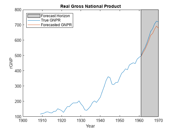
yF is a 10-by-1 vector of future values of real GNP corresponding to the future predictor data.
Estimate the forecast root mean squared error (RMSE).
frmse = sqrt(mean((yF - yFT).^2))
frmse =
25.5397
The forecast RMSE is a relative measure of forecast accuracy. Specifically, you estimate several models using different assumptions. The model with the lowest forecast RMSE is the best-performing model of the ones being compared.
Copyright 2018 The MathWorks, Inc.
More About
Algorithms
You can reset all model properties using dot notation, for example, PriorMdl.V
= diag(Inf(3,1)). For property resets, conjugateblm does
minimal error checking of values. Minimizing error checking has the
advantage of reducing overhead costs for Markov chain Monte Carlo
simulations, which results in efficient execution of the algorithm.
Alternatives
The bayeslm function can create any supported prior model object for Bayesian linear regression.
Version History
Introduced in R2017a