modalreal

Compute modal state-space realization

Since R2023b

Syntax

[msys,blks] = modalreal(sys)

[msys,blks,TL,TR] = modalreal(sys)

[___] = modalreal(sys,Name=Value)

Description

[msys,blks] = modalreal(sys) returns a modal realization msys of an LTI model sys. This is a realization where A or (A,E) are block diagonal and each block corresponds to a real pole, a complex pair, or a cluster of repeated poles. blks is a vector containing block sizes down the diagonal.

For sparse models, this syntax returns a truncated modal realization. By default, the function computes the first 1000 modes of smallest magnitude. (since R2026a)

[msys,blks,TL,TR] = modalreal(sys) also returns the block-diagonalizing transformations TL and TR.

[___] = modalreal(sys,Name=Value) returns the modal realization based on the options specified by one or more name-value arguments. Use these options for controlling the block size and normalizing 2-by-2 blocks associated with complex pairs.

For sparse models, this syntax returns a truncated modal realization based on the subset of computed poles. This subset is controlled by the Focus and MaxOrder options. (since R2026a)

Examples

Convert State-Space Model to Modal Form

pendulumCartSSModel.mat contains the state-space model of an inverted pendulum on a cart where the outputs are the cart displacement $x$ and the pendulum angle $\theta$. The control input u is the horizontal force on the cart.

$$\begin{array}{l}\left[\begin{array}{c}\underset{}{\overset{\dot{}}{x}}\\ \underset{}{\overset{¨}{x}}\\ \underset{}{\overset{\dot{}}{\theta }}\\ \underset{}{\overset{¨}{\theta }}\end{array}\right]=\left[\begin{array}{cccc}0& 1& 0& 0\\ 0& -0.1& 3& 0\\ 0& 0& 0& 1\\ 0& -0.5& 30& 0\end{array}\right]\left[\begin{array}{c}x\\ \underset{}{\overset{\dot{}}{x}}\\ \theta \\ \underset{}{\overset{\dot{}}{\theta }}\end{array}\right]+\left[\begin{array}{c}0\\ 2\\ 0\\ 5\end{array}\right]u\\ y=\left[\begin{array}{cccc}1& 0& 0& 0\\ 0& 0& 1& 0\end{array}\right]\left[\begin{array}{c}x\\ \underset{}{\overset{\dot{}}{x}}\\ \theta \\ \underset{}{\overset{\dot{}}{\theta }}\end{array}\right]+\left[\begin{array}{c}0\\ 0\end{array}\right]u\end{array}$$

First, load the state-space model sys to the workspace.

load('pendulumCartSSModel.mat','sys');

Convert sys to modal form and extract the block sizes.

[msys,blks,TL,TR] = modalreal(sys)

msys =
 
  A = 
           x1      x2      x3      x4
   x1       0       0       0       0
   x2       0   -0.05       0       0
   x3       0       0  -5.503       0
   x4       0       0       0   5.453
 
  B = 
          u1
   x1  1.875
   x2  6.298
   x3   12.8
   x4  12.05
 
  C = 
              x1         x2         x3         x4
   y1         16     -4.763  -0.003696   0.003652
   y2          0   0.003969   -0.03663    0.03685
 
  D = 
       u1
   y1   0
   y2   0
 
Continuous-time state-space model.
Model Properties

blks = 4×1

     1
     1
     1
     1

TL = 4×4

    0.0625    1.2500   -0.0000   -0.1250
         0    4.1986    0.0210   -0.4199
         0    0.2285  -13.5873    2.4693
         0   -0.2251   13.6287    2.4995

TR = 4×4

   16.0000   -4.7631   -0.0037    0.0037
         0    0.2381    0.0203    0.0199
         0    0.0040   -0.0366    0.0369
         0   -0.0002    0.2015    0.2009

msys is the modal realization of sys, blks represents the block sizes down the diagonal, and TL and TR represent the block-diagonalizing transformation matrices.

Modal Realization of Zero-Pole-Gain Model

For this example, consider the following system with doubled poles and clusters of close poles:

$$sys\left(s\right)=100\frac{\left(s-1\right)\left(s+1\right)}{s\left(s+10\right)\left(s+10.0001\right){\left(s-\left(1+i\right)\right)}^2{\left(s-\left(1-i\right)\right)}^2}$$

Create a zpk model of this system and obtain a modal realization using the function modalreal.

sys = zpk([1 -1],[0 -10 -10.0001 1+1i 1-1i 1+1i 1-1i],100);
[msys1,blks1] = modalreal(sys);
blks1

blks1 = 3×1

     1
     4
     2

msys1.A

ans = 7×7

         0         0         0         0         0         0         0
         0    1.0000    2.1220         0         0         0         0
         0   -0.4713    1.0000    1.5296         0         0         0
         0         0         0    1.0000    1.8439         0         0
         0         0         0   -0.5423    1.0000         0         0
         0         0         0         0         0  -10.0000    4.0571
         0         0         0         0         0         0  -10.0001

msys1.B

ans = 7×1

    0.1600
   -0.0052
    0.0201
   -0.0975
    0.2884
         0
    4.0095

sys has a pair of poles at s = -10 and s = -10.0001, and two complex poles of multiplicity 2 at s = 1+i and s = 1-i. As a result, the modal form msys1 is a state-space model with a block of size 2 for the two poles near s = -10, and a block of size 4 for the complex eigenvalues.

Now, separate the two poles near s = -10 by increasing the condition number of the block-diagonalizing transformation. Set SepTol to 1e-10 for this example.

[msys2,blks2] = modalreal(sys,SepTol=1e-10);
blks2

blks2 = 4×1

     1
     4
     1
     1

msys2.A

ans = 7×7

         0         0         0         0         0         0         0
         0    1.0000    2.1220         0         0         0         0
         0   -0.4713    1.0000    1.5296         0         0         0
         0         0         0    1.0000    1.8439         0         0
         0         0         0   -0.5423    1.0000         0         0
         0         0         0         0         0  -10.0000         0
         0         0         0         0         0         0  -10.0001

msys2.B

ans = 7×1
105 ×

    0.0000
   -0.0000
    0.0000
   -0.0000
    0.0000
    1.6267
    1.6267

The A matrix of msys2 includes separate diagonal elements for the poles near s = -10. Increasing the condition number results in some very large values in the B matrix.

Normalize Diagonal Blocks in Modal Realizations

For this example, consider the following system with complex pair poles and clusters of close poles:

$$sys\left(s\right)=100\frac{\left(s-1\right)\left(s+1\right)}{s\left(s+10\right)\left(s+10.0001\right){\left(s-\left(3+4i\right)\right)}^2}$$

Create a zpk model of this system and obtain a modal realization using the function modalreal.

sys = zpk([1 -1],[0 -10 -10.0001 3+4i 3-4i],100);
[msys1,blks1] = modalreal(sys);
blks1

blks1 = 3×1

     1
     2
     2

msys1.A

ans = 5×5

         0         0         0         0         0
         0    3.0000    8.7637         0         0
         0   -1.8257    3.0000         0         0
         0         0         0  -10.0000    8.8001
         0         0         0         0  -10.0001

msys1 is a state-space model with a block of sizes 2 for the two poles near s = -10, and a pair of complex poles at s = 3+4i and s = 3-4i.

You can normalize the values of 2-by-2 blocks to show the actual pole values using the Normalize option. Additionally, relax the relative accuracy of the block diagonalizing transformation to separate the block near s = -10.

[msys2,blks2] = modalreal(sys,Normalize=true,SepTol=1e-10);
blks2

blks2 = 4×1

     1
     2
     1
     1

msys2.A

ans = 5×5

         0         0         0         0         0
         0    3.0000    4.0000         0         0
         0   -4.0000    3.0000         0         0
         0         0         0  -10.0000         0
         0         0         0         0  -10.0001

For complex poles, this option normalizes the 2-by-2 block of complex poles $a\pm \text{bi}$ to $\left[\begin{array}{cc}a& b\\ -b& a\end{array}\right]$.

Compute Truncated Modal Realization of Sparse Models

Since R2026a

This example shows how to obtain a truncated modal realization for a sparse model using modalreal.

Load the sparse model.

load flowmeterSparse.mat
size(sys)

Sparse state-space model with 5 outputs, 1 inputs, and 9669 states.

The sparse model contains 9669 states. By default, modalreal computes the first 1000 poles of smallest magnitude for sparse models, which may be time consuming. Computing the modal realization, you can see that modalreal returns a realization of size 1000.

[msys,blks,TL,TR] = modalreal(sys);
size(msys)

State-space model with 5 outputs, 1 inputs, and 1000 states.

You can limit the subset of computed poles using the Focus and MaxOrder options. For example, compute the modal realization in the frequency range 0 rad/s to 250 rad/s.

[msys2,blks2,TL2,TR2] = modalreal(sys,Focus=[0 250]);
size(msys2)

State-space model with 5 outputs, 1 inputs, and 33 states.

Compare the frequency response of the truncated realizations with the original sparse model.

sigmaplot(sys,msys,".-",msys2,"--",w)
legend("Original model","Truncated realization (1000 modes)",...
    "Truncated realization (33 modes)")

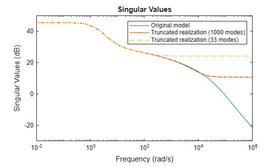
Use this workflow to quickly obtain a truncated modal realization of a sparse model. For more flexibility, first use reducespec to obtain a reduced-order model, then apply modalreal to the result.

Input Arguments

sys — Dynamic system

dynamic system model

Dynamic system, specified as a SISO, or MIMO dynamic system model. Dynamic systems that you can use include:

• Continuous-time or discrete-time numeric LTI models, such as tf (Control System Toolbox), zpk (Control System Toolbox), ss (Control System Toolbox), or pid (Control System Toolbox) models.

• Generalized or uncertain LTI models such as genss (Control System Toolbox) or uss (Robust Control Toolbox) models. (Using uncertain models requires Robust Control Toolbox™ software.)

• Identified LTI models, such as idtf, idss, idproc, idpoly, and idgrey models.

• Sparse state-space models, sparss (Control System Toolbox) or mechss (Control System Toolbox). (since R2026a)

  For sparse models, modalreal is helpful when you want to quickly obtain a truncated modal form. For more flexibility, first use reducespec (Control System Toolbox) to obtain a reduced-order model, then apply modalreal to the result.

You cannot use frequency-response data models such as frd (Control System Toolbox) models.

Name-Value Arguments

Specify optional pairs of arguments as Name1=Value1,...,NameN=ValueN, where Name is the argument name and Value is the corresponding value. Name-value arguments must appear after other arguments, but the order of the pairs does not matter.

Example: [msys,blks] = modalreal(sys,Normalize=true)

SepTol — Relative accuracy of block diagonalization

1e-12 (default) | scalar between 0 and 1

Relative accuracy of block diagonalization, specified as a scalar between 0 and 1.

This option limits the condition number of the block diagonalizing transformation to roughly SepTol/eps. Increasing SepTol helps yield smaller blocks at the expense of accuracy.

Normalize — Normalize diagonal blocks

false or 0 (default) | true or 1

Normalize 1-by-1 and 2-by-2 diagonal blocks, specified as a logical 0 (false) or 1 (true).

When Normalize is true, the function normalizes the block to show the pole values.

• For explicit models, the function normalizes 2-by-2 blocks associated with complex pairs a±jb to $$\left[\begin{array}{cc}a& b\\ -b& a\end{array}\right]$$.

• For descriptor models, the function normalizes

  • 1-by-1 blocks to A_j = a, E_j = 1.

  • 2-by-2 blocks to A_j = $$\left[\begin{array}{cc}a& b\\ -b& a\end{array}\right]$$, E_j = I.

Focus — Frequency range of interest

[0 inf] (default) | vector

Since R2026a

Frequency range of interest, specified as a vector of form [fmin,fmax]. When you specify a value for this property, the algorithm computes only modes in this frequency range.

By default, the focus is unspecified ([0 inf]) and the algorithm computes the MaxOrder modes with smallest magnitude.

MaxOrder — Maximum order of modal approximation

1000 (default) | positive integer

Since R2026a

Maximum order of the modal approximation, specified as a positive integer. This value limits the number of eigenvalues computed by the Krylov-Schur iterations ([1] (Control System Toolbox)) and the order of the modal approximation of the original sparse model.

ModeTol — Accuracy of computed modes

1e-12 (default) | positive scalar

Since R2026a

Tolerance for identifying converged eigenvalues in Krylov-Schur iterations, specified as a positive scalar.

DCFrequency — Frequency for evaluating DC contribution

0 (default) | nonnegative scalar

Since R2026a

Frequency for evaluating and matching DC contributions, specified as a nonnegative scalar.

For models with integrators, you cannot evaluate modal contributions at DC since the DC gain is infinite. To evaluate modal contributions and match gains at a different frequency, set the property to a positive value. The default value of this property corresponds to the true DC value.

InputScaling — Input scaling

[] (default) | vector

Since R2026a

Input scaling factors, specified as a vector of length Nu, where Nu is the number of inputs in the original model sys.

Use this option to emphasize specific input channels in sys. The software evaluates the modal contributions for the scaled system.

OutputScaling — Output scaling

[] (default) | vector

Since R2026a

Output scaling factors, specified as a vector of length Ny, where Ny is the number of outputs in the original model sys.

Use this option to emphasize specific output channels in sys. The software evaluates the modal contributions for the scaled system.

Display — Show or hide progress report

"on" (default) | "off"

Since R2026a

Show or hide progress report, specified as either "off" or "on".

Output Arguments

msys — Modal state-space realization

ss model object

Modal state-space realization of the dynamic model, returned as an ss (Control System Toolbox) model object. msys is a realization where A or (A,E) are block diagonal and each block corresponds to a real pole, a complex pair, or a cluster of repeated poles.

blks — Block sizes

vector

Block sizes in the block-diagonal realization, returned as a vector.

TL — Left-side matrix of block-diagonalizing transformation

matrix | []

Left-side matrix of the block-diagonalizing transformation, returned as a matrix.

• For ordinary LTI models, TL is a matrix of size Nx-by-Nx, where Nx is the number of states in the model sys

• For sparse models, TL is a matrix of size n_c-by-Nx, where n_c is the number of computed modal components. For mechss models, TL corresponds to the equivalent first-order representation sparss(sys). (since R2026a)

The algorithm transforms the state-space realization (A, B, C, D, E) of a model to block diagonal matrices (A_m, B_m, C_m, D_m, E_m) given by:

• For explicit state-space models

  $$\begin{array}{l}\begin{array}{cc}{A}_m=T_{L}A{T}_R,& B_m=T_{L}B,\end{array}\\ \begin{array}{ccc}{C}_m=C{T}_R,& D_m=D,& E=T_L{T}_R=I\end{array}\end{array}$$

• For descriptor state-space models

  $$\begin{array}{l}\begin{array}{cc}{A}_m=T_{L}A{T}_R,& B_m=T_{L}B,\end{array}\\ \begin{array}{ccc}{C}_m=C{T}_R,& D_m=D,& E_m=T_{L}E{T}_R\end{array}\end{array}$$

The function returns an empty value [] for this argument when the input model sys is not a state-space model.

TR — Right-side matrix of block-diagonalizing transformation

matrix | []

Right-side matrix of the block-diagonalizing transformation, returned as a matrix.

• For ordinary LTI models, TR is a matrix of size Nx-by-Nx, where Nx is the number of states in the model sys

• For sparse models, TR is a matrix of size Nx-by-n_c, where n_c is the number of computed modal components. For mechss models, TR corresponds to the equivalent first-order representation sparss(sys). (since R2026a)

The algorithm transforms the state-space realization (A, B, C, D, E) of a model to block diagonal matrices (A_m, B_m, C_m, D_m, E_m) given by:

• For explicit state-space models

  $$\begin{array}{l}\begin{array}{cc}{A}_m=T_{L}A{T}_R,& B_m=T_{L}B,\end{array}\\ \begin{array}{ccc}{C}_m=C{T}_R,& D_m=D,& E=T_L{T}_R=I\end{array}\end{array}$$

• For descriptor state-space models

  $$\begin{array}{l}\begin{array}{cc}{A}_m=T_{L}A{T}_R,& B_m=T_{L}B,\end{array}\\ \begin{array}{ccc}{C}_m=C{T}_R,& D_m=D,& E_m=T_{L}E{T}_R\end{array}\end{array}$$

The function returns an empty value [] for this argument when the input model sys is not a state-space model.

References

[1] Stewart, G. W. “A Krylov--Schur Algorithm for Large Eigenproblems.” SIAM Journal on Matrix Analysis and Applications 23, no. 3 (January 2002): 601–14. https://doi.org/10.1137/S0895479800371529.

Version History

Introduced in R2023b

R2026a: Support for Sparse Models: Compute truncated modal form

You can now use modalreal to compute a truncated modal form of sparse state-space models. This is helpful when you want to quickly obtain a truncated modal form of sparse models.

For more flexibility, first use reducespec (Control System Toolbox) to obtain a reduced-order model, then apply modalreal to the result.