Spectrum Sensing with Deep Learning for Radar and Wireless Communications
This example shows how to perform spectrum sensing using a semantic segmentation neural network trained with synthesized radar and wireless communication signals. The trained neural network can identify radar and wireless communication signals that appear in the same received spectrum. In addition, the network can identify the occupied bandwidth of the received signals.
Introduction
Due to the increasing demands for higher speeds and greater coverage, modern wireless communication systems are moving to higher frequency bands and larger signal bandwidths. These higher frequency bands are at ranges traditionally used by radar systems. As a result, the spectrum of radar systems and wireless communication systems may overlap, which drives the need for spectrum sharing. This requires that future radar and wireless communication systems include spectrum sensing to detect occupied space to avoid conflicts. This example shows how to model a spectrum sensing system. We first synthesize a data set that consists of radar and wireless communications signals. This data is used to train and test a deep learning network. The trained network is then used to identify the signals and the corresponding occupied bandwidth of these signals.
Setup the Scene
Consider an airport surveillance radar located at the scenario origin. The radar operates at 2.8 GHz and uses a reflector antenna with a gain of 32.8 dB. The transmit power is set at 25 kW.
% setup waveform
fc=2.8e9;                   % center frequency [Hz]
fs=61.44e6;                 % sampling frequency [Hz]
prf=fs/ceil(fs/1050);       % pulse repetition rate [Hz]
pulseWidth=1e-06;           % pulsewdith [s]
wav = phased.RectangularWaveform('SampleRate',fs,'PulseWidth',pulseWidth,'PRF',prf,'NumPulses',3);

% setup antenna
rad=2.5;            % radius [m]
flen=2.5;           % focal length [m]
antele=design(reflectorParabolic('Exciter',horn),fc);
antele.Exciter.Tilt=90;
antele.Exciter.TiltAxis=[0 1 0];
antele.Tilt=90;
antele.TiltAxis=[0 1 0];
antele.Radius=rad;
antele.FocalLength=flen;
ant=phased.ConformalArray('Element',antele);

% setup transmitter and receiver
power_ASR=25000;    % transmit power [W]
gain_ASR=32.8;      % transmit gain [dB]
radartx = phased.Transmitter('PeakPower',power_ASR,'Gain',gain_ASR);
Since 5G and LTE signals are present in the vicinity of airport radars, we define a set of signals for these wireless standards using 5G Toolbox and LTE Toolbox. For more details on how to generate these types of signals, refer to the example "Spectrum Sensing with Deep Learning to Identify 5G and LTE Signals".
For the wireless signals, the gain and the power of the transmitter may change from frame to frame. The receivers are assumed to be randomly placed in a 2 km x 2km region and equipped with isotropic antennas.
rxpos_horiz_minmax=[-1000 1000];
rxpos_vert_minmax=[0 2000];
The region also contains many scatterers which makes the propagation channels more challenging to operate in. In this example, we assume the channel contains 30 scatterers, randomly distributed in the region. You can use phased.ScatteringMIMOChannel to simulate the scatterers.
% define radar position
radartxpos=[0 0 15]';
radartxaxes=rotz(0);
radarchan=phased.ScatteringMIMOChannel('TransmitArray',ant,...
    'ReceiveArray',phased.ConformalArray('Element',phased.IsotropicAntennaElement),...
    'CarrierFrequency',fc,...
    'SpecifyAtmosphere',true,...
    'SampleRate',fs,...
    'SimulateDirectPath',false,...
    'MaximumDelaySource','Property',...
    'MaximumDelay',1,...
    'TransmitArrayMotionSource','Property',...
    'TransmitArrayPosition',radartxpos,...
    'TransmitArrayOrientationAxes',radartxaxes,...
    'ReceiveArrayMotionSource','Input port',...
    'ScattererSpecificationSource','Input port');

% define wireless transmitter position
commtxpos=[200 0 450]';
commtxaxes=rotz(0);
commchan=phased.ScatteringMIMOChannel('TransmitArray',phased.ConformalArray('Taper',10),...
    'ReceiveArray',phased.ConformalArray('Element',phased.IsotropicAntennaElement),...
    'CarrierFrequency',fc,...
    'SpecifyAtmosphere',true,...
    'SampleRate',fs,...
    'SimulateDirectPath',false,...
    'MaximumDelaySource','Property',...
    'MaximumDelay',1,...
    'TransmitArrayMotionSource','Property',...
    'TransmitArrayPosition',commtxpos,...
    'TransmitArrayOrientationAxes',commtxaxes,...
    'ReceiveArrayMotionSource','Input port',...
    'ScattererSpecificationSource','Input port');
Generate Training Data
To generate the training data, define the data folder and class names for noise only data, LTE data, 5G NR data, and radar data. Because we are looking for the waveform type and the occupied bandwidth, the helper function below generates a spectrogram.
% Number of data generated
numTrainingData=500;
imageSize=[256 256];

% Define data directory
classNames = ["Noise" "LTE" "NR" "Radar"];
pixelLabelID = [0 1 2 3];
useDownloadedDataSet = true;
saveFolder = tempdir;
trainingFolder=fullfile(saveFolder,'RadarCommTrainData');
if ~useDownloadedDataSet
    % Generate data
    helperGenerateRadarCommData(fs,wav,radartx,radarchan,commchan,rxpos_horiz_minmax,rxpos_vert_minmax,numTrainingData,trainingFolder,imageSize);
else
    dataURL = 'https://ssd.mathworks.com/supportfiles/phased/data/RadarCommSpectrumSensingData.zip';
    zipFile = fullfile(saveFolder,'RadarCommSpectrumSensingData.zip');
    if ~exist(zipFile,'file')
        websave(zipFile,dataURL);
        % Unzip the data
        unzip(zipFile,saveFolder)
    end
end
Load Training Data
Use the imageDatastore function to load training images with the spectrogram of radar and wireless communication signals. The imageDatastore function enables you to efficiently load a large collection of images from disk. Spectrogram images are stored in .png files.
% Data
trainingFolder = fullfile(saveFolder,'RadarCommTrainData');
imds = imageDatastore(trainingFolder,'IncludeSubfolders',false,'FileExtensions','.png');
To label the occupied bandwidth for each signal, use the pixelLabelDatastore (Computer Vision Toolbox) function to load spectrogram pixel label image data. Each pixel in the spectrogram images is labeled as one of "Radar", "NR", "LTE" or "Noise" categories. A pixel label datastore encapsulates the pixel label data and the label ID to a class name mapping. Pixel labels are stored in .hdf files.
% Label
pxdsTruth = pixelLabelDatastore(trainingFolder,classNames,pixelLabelID,...
  'IncludeSubfolders',false,'FileExtensions','.hdf');
Analyze Dataset Statistics
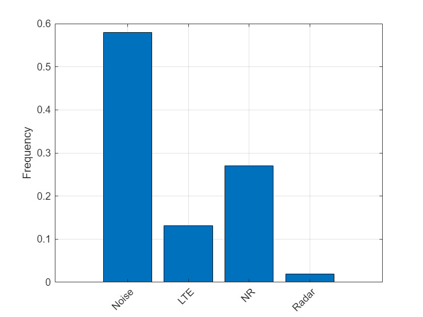
To see the distribution of class labels in the training dataset, use the countEachLabel (Computer Vision Toolbox) function to count the number of pixels by class label, and plot the pixel counts by class.
tbl = countEachLabel(pxdsTruth);
frequency = tbl.PixelCount/sum(tbl.PixelCount);
figure
bar(1:numel(classNames),frequency)
grid on
xticks(1:numel(classNames))
xticklabels(tbl.Name)
xtickangle(45)
ylabel('Frequency')

Prepare Training, Validation, and Test Sets
The deep neural network uses 80% of the single signal images from the dataset for training and, 20% of the images for validation. The helperSpecSensePartitionData function randomly splits the image and pixel label data into training and validation sets.
[imdsTrain,pxdsTrain,imdsVal,pxdsVal] = helperRadarCommPartitionData(imds,pxdsTruth,[80 20]);
cdsTrain = combine(imdsTrain,pxdsTrain);
cdsVal = combine(imdsVal,pxdsVal);
Train Deep Neural Network
Use the deeplabv3plus (Computer Vision Toolbox) function to create a semantic segmentation neural network. Choose resnet50 (Deep Learning Toolbox) as the base network and specify the input image size (number of pixels used to represent time and frequency axes) and the number of classes. If the Deep Learning Toolbox™ Model for ResNet-50 Network support package is not installed, then the function provides a link to the required support package in the Add-On Explorer. To install the support package, click the link, and then click Install. Check that the installation is successful by typing resnet50 at the command line. If the required support package is installed, then the function returns a Make Predictions Using dlnetwork Object (Deep Learning Toolbox) object.
baseNetwork = 'resnet50';
lgraph = deeplabv3plus(imageSize,numel(classNames),baseNetwork);
Balance Classes Using Class Weighting
To improve training when classes in the training set are not balanced, you can use class weighting to balance the classes. Use the pixel label counts computed earlier with the countEachLabel function and calculate the median frequency class weights.
imageFreq = tbl.PixelCount ./ tbl.ImagePixelCount;
classWeights = median(imageFreq) ./ imageFreq;
classWeights = classWeights/(sum(classWeights)+eps(class(classWeights)));
Select Training Options
Configure training using the trainingOptions (Deep Learning Toolbox) function to specify the stochastic gradient descent with momentum (SGDM) optimization algorithm and the hyper-parameters used for SGDM. To get the best performance from the network, you can use the Experiment Manager (Deep Learning Toolbox) to optimize training options.
opts = trainingOptions("sgdm",...
  MiniBatchSize = 40,...
  MaxEpochs = 40, ...
  LearnRateSchedule = "piecewise",...
  InitialLearnRate = 0.02,...
  LearnRateDropPeriod = 10,...
  LearnRateDropFactor = 0.1,...
  ValidationData = cdsVal,...
  ValidationPatience = 5,...
  Shuffle="every-epoch",...
  Plots = "training-progress",...
  OutputNetwork = "best-validation-loss",...
  Metrics = "accuracy",...
  ExecutionEnvironment = "auto");
Train the network using the combined training data store, cdsTrain. The combined training data store contains single signal frames and true pixel labels. Use weighted cross-entropy loss together with a custom normalization to update the network during training. Define a custom loss function, helperWeightedCrossEntropyLoss, using the crossentropy (Deep Learning Toolbox) loss function and apply custom normalization. One example of training progress is shown in the following figure.

If you want to train the network, set trainNow to true. Otherwise, the example will load a pre-trained network.
trainNow = false;
if trainNow
  [net,trainInfo] = trainnet(cdsTrain,lgraph,...
       @(ypred,ytrue) helperWeightedCrossEntropyLoss(ypred,ytrue,classWeights),opts);  %#ok<UNRCH>
else
  load(fullfile(saveFolder,'helperRadarCommTrainedNet.mat'),'net');
end
Test with Synthetic Signals
Test the network signal identification performance using signals that contain 5G NR, LTE, and radar signals. Use the semanticseg (Computer Vision Toolbox) function to get the pixel estimates of the spectrogram images in the test data set. Use the evaluateSemanticSegmentation (Computer Vision Toolbox) function to compute various metrics to evaluate the quality of the semantic segmentation results.
% Generate testing data
numTestData=100;
testFolder = fullfile(saveFolder,'RadarCommTestData');
if ~useDownloadedDataSet
    helperGenerateRadarCommData(fs,wav,radartx,radarchan,commchan,rxpos_horiz_minmax,rxpos_vert_minmax,numTestData,testFolder,imageSize);
end
% Prep and test the testing data
imds = imageDatastore(testFolder,'IncludeSubfolders',false,'FileExtensions','.png');
pxdsResults = semanticseg(imds,net,"WriteLocation",saveFolder, ...
    'Classes',classNames,'ExecutionEnvironment','auto');
Running semantic segmentation network
-------------------------------------
* Processed 588 images.
% Prep the ground truth testing labels
pxdsTruth = pixelLabelDatastore(testFolder,classNames,pixelLabelID,...
  'IncludeSubfolders',false,'FileExtensions','.hdf');
metrics = evaluateSemanticSegmentation(pxdsResults,pxdsTruth);
Evaluating semantic segmentation results
----------------------------------------
* Selected metrics: global accuracy, class accuracy, IoU, weighted IoU, BF score.
* Processed 588 images.
* Finalizing... Done.
* Data set metrics:

    GlobalAccuracy    MeanAccuracy    MeanIoU    WeightedIoU    MeanBFScore
    ______________    ____________    _______    ___________    ___________

       0.89313          0.91483       0.70508      0.81645        0.83124
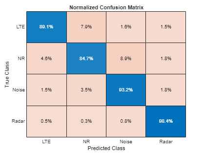
Plot the normalized confusion matrix for all test frames.
cm = confusionchart(metrics.ConfusionMatrix.Variables, ...
  classNames, Normalization='row-normalized');
cm.Title = 'Normalized Confusion Matrix';

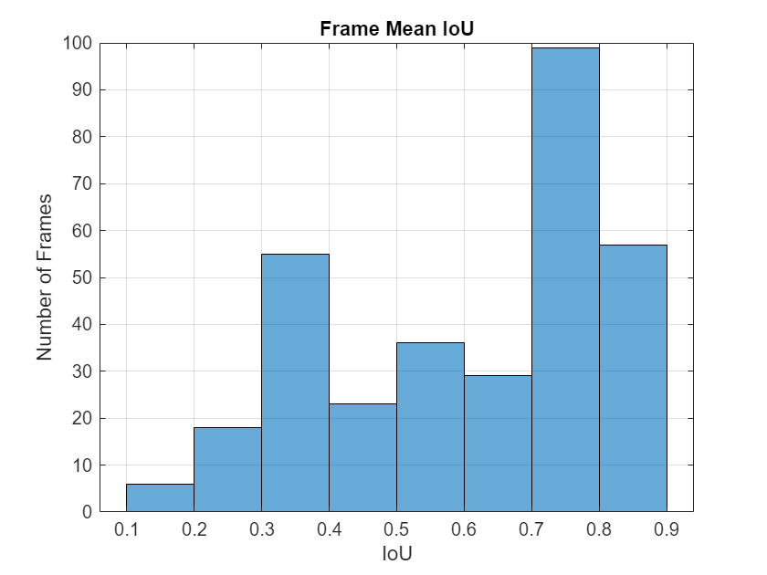
Plot the histogram of the per-image intersection over union (IoU). For each class, IoU is the ratio of correctly classified pixels to the total number of ground truth and predicted pixels in that class.
imageIoU = metrics.ImageMetrics.MeanIoU;
figure
histogram(imageIoU)
grid on
xlabel('IoU')
ylabel('Number of Frames')
title('Frame Mean IoU')

Identify Radar, 5G NR, and LTE Signals in Spectrogram
Visualize the received spectrum, true labels, and predicted labels for the image with index 142. We can see that the network correctly picked out the radar signal from wireless communication signals.
imgIdx = 142;
rcvdSpectrogram = readimage(imds,imgIdx);
trueLabels = readimage(pxdsTruth,imgIdx);
predictedLabels = readimage(pxdsResults,imgIdx);
figure
helperSpecSenseDisplayResults(rcvdSpectrogram,trueLabels,predictedLabels, ...
  classNames,fs,0,1/prf)
Conclusions
The trained network can distinguish radar and wireless communication signals. The network may not be able to identify every captured signal correctly. In such cases, enhance the training data either by generating more representative synthetic signals or capturing over-the-air signals and including these in the training set.