Creare un modello semplice

È possibile usare Simulink^® per modellare un sistema e poi simularne il comportamento dinamico. In questo esempio si crea un modello semplice, ma è possibile utilizzare le stesse tecniche di base per creare modelli complessi. L'esempio simula il movimento semplificato di un'automobile. Di solito un'automobile è in movimento fintanto che viene premuto il pedale dell'acceleratore. Una volta rilasciato il pedale, l'auto rallenta fino a fermarsi e rimane al minimo.

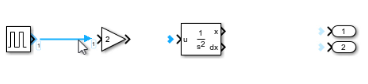
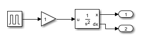
Un blocco Simulink è l'elemento del modello che definisce una relazione matematica tra i suoi input e output. Per creare questo semplice modello, sono necessari quattro blocchi Simulink.

Nome del blocco	Scopo del blocco	Scopo del modello
Pulse Generator	Generare un segnale di input per il modello.	Rappresentare il pedale dell'acceleratore.
Gain	Moltiplicare il segnale di input per un valore costante.	Calcolare in che modo la pressione sull'acceleratore influisce sull'accelerazione dell'auto.
Second-Order Integrator	Integrare due volte il segnale di input.	Ottenere la posizione dall'accelerazione.
Outport	Designare un segnale come output del modello.	Designare la posizione come output del modello.

La simulazione di questo modello integra due volte un breve impulso per ricreare una rampa. L'impulso di input rappresenta una pressione del pedale dell'acceleratore: 1 quando il pedale viene premuto e 0 quando non lo è. La rampa di output rappresenta la distanza crescente dal punto di partenza.

Aprire un nuovo modello

Utilizzare Simulink Editor per costruire i modelli.

1. Avviare MATLAB^®. Dalla barra degli strumenti di MATLAB, fare clic sul pulsante Simulink .

   

2. Selezionare il template Blank Model.

   Si apre l'editor di Simulink.

   Per evitare il shadowing, ossia l'apertura simultanea di più modelli con lo stesso nome, l'Editor di Simulink controlla i modelli e i file caricati sul percorso e crea un modello con il nome successivo disponibile: untitled, untitled1, untitled2 e così via.

   

3. Nella scheda Simulation, selezionare Save > Save as. Nella casella di testo File name, inserire un nome per il modello, ad esempio simple_model. Fare clic su Save. Il modello viene salvato con l'estensione del file .slx.

Aprire il browser delle librerie di Simulink

Simulink fornisce un insieme di librerie di blocchi che sono organizzate per funzionalità nel Library Browser. Queste librerie si trovano nella maggior parte dei workflow:

• Continui: blocchi di sistemi con stati continui

• Discreti: blocchi di sistemi con stati discreti

• Operazioni matematiche: blocchi che implementano equazioni algebriche e logiche

• Sink: blocchi che memorizzano e mostrano i segnali che si collegano a loro

• Sorgenti: blocchi che generano i valori dei segnali che guidano il modello

Per aprire il browser delle librerie, sulla barra degli strumenti di Simulink, nella scheda Simulation, fare clic su Library Browser.

Per sfogliare le librerie di blocchi, nella struttura ad albero delle librerie, espandere una libreria e le relative sottolibrerie.

Per cercare tutte le librerie dii blocchi disponibili, inserire un termine di ricerca. Ad esempio, trovare il blocco Pulse Generator. Nella finestra di ricerca, inserire pulse, quindi premere Invio. Il software cerca nelle librerie i blocchi con pulse nel nome o nella descrizione e poi li mostra nella scheda Search Results del browser delle librerie. È possibile ritornare a sfogliare la struttura ad albero delle librerie facendo clic sulla scheda Library.

Aggiunta di blocchi al modello

Per iniziare a costruire il modello, si aggiungono blocchi all'area di disegno del modello. È possibile aggiungere blocchi utilizzando il browser delle librerie o il menu di inserimento rapido.

1. Aggiungere un blocco Pulse Generator. Nella struttura ad albero del browser delle librerie, espandere la libreria di Simulink. Espandere la sottolibreria Sources. Trascinare il blocco Pulse Generator nell'area di disegno del modello.

   

2. Aggiungere un blocco Gain. Fare doppio clic sull'area di disegno del modello. Nel menu di inserimento rapido visualizzato, inserire gain. Si visualizza un elenco di blocchi.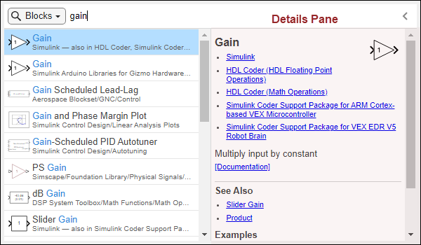

   

   Possono esistere più blocchi con lo stesso nome, purché siano memorizzati in file diversi della libreria. Le librerie a cui appartiene un blocco sono elencate sotto il nome del blocco. Verificare che il blocco Gain della libreria di Simulink sia selezionato. Qualora non lo fosse, utilizzare i tasti freccia o fare clic sul nome del blocco.

   Per saperne di più sul blocco selezionato, leggere la descrizione nel pannello dei dettagli, a destra dei risultati della ricerca. Per consultare la documentazione completa relativa al blocco, fare clic su Documentation. Per alcuni esempi relativi al blocco, fare clic sui collegamenti sotto Examples. Per nascondere o mostrare il pannello dei dettagli, fare clic sulla freccia in alto a destra.

   Aggiungere il blocco selezionato al modello premendo INVIO o facendo doppio clic sulla selezione.

   

3. Aggiungere questi blocchi al modello utilizzando il browser delle librerie o il menu di inserimento rapido.

   Blocco	Libreria
   Out1	Libreria di Simulink, sottolibreria Sinks
   Second-Order Integrator	Libreria di Simulink, sottolibreria Continuous

4. Aggiungere un secondo blocco Out1 copiando quello esistente e incollandolo in un altro punto utilizzando le scorciatoie da tastiera CTRL+C e CTRL+V (su macOS, utilizzare Comando+C e Comando+V). Ora il modello possiede tutti i blocchi necessari.

Collegare i blocchi

Collegare il:

• Blocco Pulse Generator al blocco Gain.

• Blocco Gain al blocco Second-Order Integrator.

• Blocco Second-Order Integrator ai due blocchi Out1.

Ad esempio, per collegare il blocco Pulse Generator al blocco Gain:

1. Fare clic sulla porta di output a destra del blocco Pulse Generator.

   La porta di output e tutte le porte di input che possono essere collegate sono indicate dal simbolo di una freccia blu (>).

2. Per vedere l’indicazione del collegamento, puntare il simbolo della freccia (>).

3. Fare clic sulla spunta per collegare i blocchi con una linea e una freccia che indica la direzione del flusso del segnale.

Per ulteriori informazioni su come collegare i blocchi, vedere Connect Blocks.

Una volta collegati i blocchi, allineare i blocchi Pulse Generator, Gain e Second-Order Integrator trascinandoli. Per ridimensionare un blocco, trascinarne un angolo.

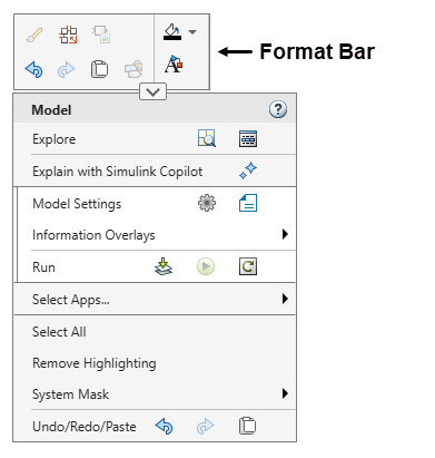
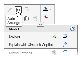
Per i modelli di grandi dimensioni, anziché trascinare i singoli blocchi, è possibile migliorare il layout del modello utilizzando la disposizione automatica. Fare clic con il tasto destro del mouse sull'area di disegno del modello. Viene visualizzato il menu contestuale Top Model. Nei menu contestuali di Simulink, le opzioni di formattazione, come la modifica dei colori o dei caratteri o la disposizione automatica del modello, si trovano nella barra di formattazione. Per espandere la barra di formattazione, nella parte superiore del menu, fare clic sulla freccia . Quindi, fare clic sul pulsante Auto Arrange (Disposizione automatica) .

Suggerimento

Per visualizzare una tooltip che spiega quali operazioni è possibile eseguire premendo un pulsante del menu contestuale, soffermarsi con il puntatore del mouse sull'icona del pulsante.

La disposizione automatica allinea i blocchi e raddrizza le linee di segnale.

Modifica dei valori dei parametri del blocco

I blocchi presentano valori dei parametri che è possibile modificare. Per identificare quali parametri è possibile modificare in un blocco e quali tipi di valore possono assumere, aprire la documentazione del blocco. Fare clic con il tasto destro del mouse sul blocco e, nell'angolo in alto a destra del menu contestuale, fare clic sul pulsante Open help documentation (Apri la documentazione della guida) .

Per alcuni blocchi, come i blocchi Constant o i blocchi Gain, è possibile modificare il valore di un parametro direttamente sulla faccia del blocco. Modificare il valore di guadagno del blocco Gain nel modello di esempio in 2. Selezionare il blocco, fare clic sul valore nel blocco, inserire il nuovo valore, quindi premere INVIO.

È inoltre possibile modificare il valore del guadagno nella finestra di dialogo Block Parameters (Parametri del blocco). Per aprire la finestra di dialogo Block Parameters (Parametri del blocco), fare doppio clic sul blocco. In alternativa, fare clic con il tasto destro del mouse sul blocco, quindi fare clic sul pulsante (Parametri del blocco) . Nella finestra di dialogo che si apre, modificare il valore Gain in 2 e premere INVIO.

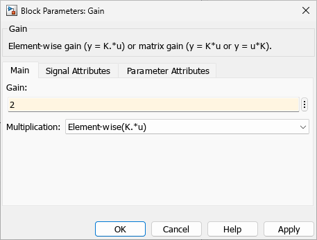
Una terza opzione consiste nell'utilizzare il Property Inspector. Selezionare il blocco Gain. Per aprire il Property Inspector, premere CTRL+MAIUSC+I (su macOS, premere Comando+Opzione+O). In alternativa, fare clic con il tasto destro del mouse sul blocco, quindi fare clic sul pulsante Property Inspector . Nel Property Inspector, nella scheda Parameters, modificare il valore di Gain in 2.

Per modificare i valori dei parametri non visualizzati sull'icona del blocco, utilizzare la finestra di dialogo Block Parameters (Parametri del blocco) o il Property Inspector. Se nella finestra di dialogo Block Parameters (Parametri del blocco) non compare il nome di un parametro di cui si desidera modificare il valore, controllare il Property Inspector e viceversa.

Eseguire una simulazione

Specificare il tempo di arresto della simulazione. Quindi, simulare il modello.

1. Nella scheda Simulation, impostare il tempo di arresto della simulazione. Sulla barra degli strumenti di Simulink, nella scheda Simulation, inserire il valore nel campo Stop Time.

   

   Il tempo di arresto predefinito di 10.0 è appropriato per questo modello. Questo valore di tempo non ha unità. L'unità di tempo in una simulazione di Simulink dipende da come sono costruite le equazioni. Questo esempio simula il movimento semplificato di un'automobile per 10 secondi ma, altri modelli, potrebbero avere unità di tempo di millisecondi o di anni.

2. Per simulare il modello, premere CTRL+T (su macOS, premere Comando+T). In alternativa, nella barra degli strumenti, nella scheda Simulation, fare clic su Run .

Visualizzazione dei dati di simulazione

Per visualizzare i risultati della simulazione in Simulation Data Inspector, fare clic con il tasto destro del mouse su una delle linee del segnale, quindi fare clic sul pulsante View in Data Inspector (Visualizza nel Data Inspector) .

Per tracciare i dati in Simulation Data Inspector, selezionare i segnali dall'elenco a sinistra. Ad esempio, per tracciare la posizione dell'automobile, selezionare il segnale denominato Out1:1.

Perfezionare il modello

È possibile perfezionare un modello modificando i parametri dei blocchi, aggiungendo nuovi blocchi, creando nuovi collegamenti e annotando le linee del segnale.

Modificare i parametri dei blocchi

Questo esempio modella un sensore di prossimità basato su un modello di movimento esistente, denominato moving_car.

In questo scenario, un sensore digitale misura la distanza tra l'automobile e un ostacolo a 10 m di distanza. Il modello emette la misura del sensore e la posizione dell'automobile, prendendo in considerazione queste condizioni:

• L'automobile si ferma bruscamente quando raggiunge l'ostacolo.

• Nel mondo fisico, un sensore misura la distanza in modo impreciso, causando errori numerici casuali.

• Un sensore digitale funziona a intervalli di tempo fissi.

Aprire il modello moving_car.

open_system("moving_car.slx");

È necessario innanzitutto modellare l'arresto brusco quando l'automobile raggiunge la posizione 10. Il blocco Integrator, Second-Order possiede un parametro apposito.

1. Fare doppio clic sul blocco Integrator, Second-Order. Appare la finestra di dialogo Parametri dei blocchi.

2. Selezionare Limite x e inserire 10 per Limite superiore x. Il colore di sfondo del parametro cambia per indicare una modifica che non viene applicata al modello. Fare clic su OK per applicare le modifiche e chiudere la finestra di dialogo.

Aggiungere nuovi blocchi e collegamenti

Modificare il modello per aggiungere un sensore che misuri la distanza dall'ostacolo. Se necessario, espandere la finestra per inserire i nuovi blocchi.

• Per trovare la distanza tra il veicolo e la posizione dell'ostacolo, aggiungere un blocco Constant della libreria Sources e impostare il valore del blocco su 10. Per trovare la distanza tra la posizione dell'ostacolo e la posizione del veicolo, aggiungere il blocco Subtract della libreria Math Operations.

• Per simulare le misurazioni imperfette di un sensore reale, aggiungere rumore al modello utilizzando il blocco Band-Limited White Noise della libreria Sources. Fare doppio clic sul blocco per impostare il parametro Noise power su 0.001. Aggiungere il rumore alla misurazione della distanza utilizzando un blocco Add della libreria Math Operations.

• In Simulink, il campionamento di un segnale a un dato intervallo richiede un sample and hold. Aggiungere il blocco Zero-Order Hold della libreria Discrete. Quindi, fare doppio clic sul blocco per modificare il parametro Sample Time su 0.1.

• Per registrare l'output del sensore, collegare il blocco Zero-Order Hold a un altro blocco Outport.

Collegare i nuovi blocchi. L'output del blocco Second-Order Integrator è già collegato a un'altra porta. Per creare una diramazione in quel segnale, fare clic con il tasto sinistro del mouse sul segnale per evidenziare le potenziali porte di collegamento e fare clic sulla porta appropriata.

Annotare i segnali

Aggiungere i nomi dei segnali al modello.

1. Fare doppio clic sul segnale e digitare il nome del segnale.

   

2. Per terminare, fare clic al di fuori della casella di testo.

3. Ripetere questi passaggi per aggiungere i nomi come illustrato.

   

Visualizzazione di segnali multipli

Confrontare il segnale actual distance con il segnale measured distance. Il segnale measured distance viene registrato come output. Per registrare il segnale actual distance, è possibile contrassegnarlo per la registrazione del segnale. Fare clic con il tasto destro del mouse sulla linea del segnale, quindi fare clic sul pulsante Log Signals (Registra segnali) . Un badge di registrazione indica che il segnale è contrassegnato per la registrazione.

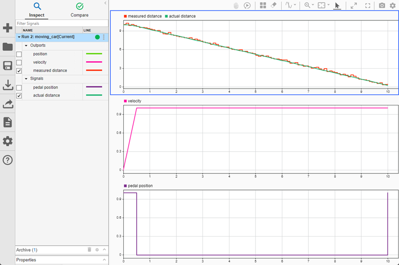
Simulare il modello. Per visualizzare i risultati della simulazione in Simulation Data Inspector, fare clic con il tasto destro del mouse sulla linea del segnale, quindi fare clic sul pulsante View in Data Inspector (Visualizza nel Data Inspector) . Espandere le liste di controllo Outports e Signals. Per tracciare entrambi i segnali sullo stesso grafico temporale, selezionare i segnali actual distance e measured distance.

Il grafico mostra che la misurazione può discostarsi dal valore effettivo fino a 0,3 m. Queste informazioni sono utili quando si progettano le feature di sicurezza, ad esempio un allarme di collisione.

Visualizzazione dei segnali su grafici secondari separati

È inoltre possibile analizzare i risultati visualizzando i segnali su grafici secondari separati. Ad esempio, è possibile aggiungere grafici secondari per i segnali pedal position e velocity per visualizzare la relazione tra la posizione del pedale, la velocità dell'automobile e la distanza tra l'automobile e l'ostacolo.

Contrassegnare il segnale pedal position per la registrazione del segnale. Fare clic con il tasto destro del mouse sulla linea del segnale pedal position, quindi fare clic sul pulsante Log Signals (Registra segnali) .

Simulare il modello. Al termine della simulazione, in Simulation Data Inspector, fare clic su Visualizations and layouts (Visualizzazioni e layout) . Quindi, creare un layout 3×1 specificando il numero di righe e colonne nella griglia.

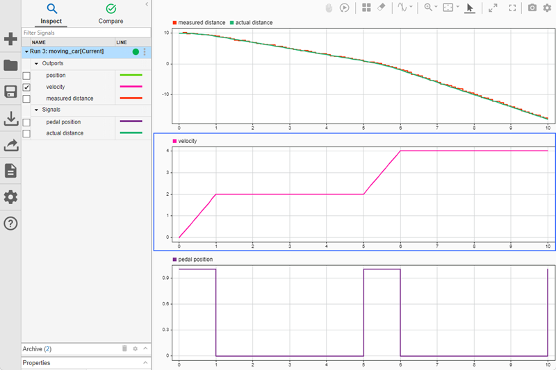
Aggiungere il segnale velocity al grafico secondario centrale e il segnale pedal position al grafico secondario inferiore. Per aggiungere un segnale a un grafico secondario, selezionare il grafico interessato, quindi il segnale dalla tabella dei segnali.

Visualizzando i dati su tre grafici secondari è possibile vedere come la pressione sul pedale dell'acceleratore influisca sulla velocità dell'automobile e sulla distanza della stessa dall'ostacolo. Per scoprire ulteriormente questo punto, è possibile modificare il comportamento del pedale dell'acceleratore regolando i parametri del blocco Pulse Generator. Per aprire la finestra di dialogo Block Parameters (Parametri del blocco) del blocco Pulse Generator, fare doppio clic sul blocco stesso. Ad esempio, impostando Period su 5 e Pulse Width su 20, il modello preme il pedale dell'acceleratore due volte per un secondo.

Simulare il modello. In Simulation Data Inspector, premere la barra spaziatrice per adattare i segnali alla visualizzazione.

In Simulation Data Inspector è possibile esaminare ulteriormente i dati personalizzando il grafico e l'aspetto dei segnali, eseguendo lo zoom e la panoramica, nonché aggiungendo cursori dati. Per ulteriori informazioni, vedere Create Plots Using the Simulation Data Inspector.

Vedi anche

Blocchi

• Pulse Generator | Gain | Second-Order Integrator | Sum | Constant | Zero-Order Hold | Band-Limited White Noise

Strumenti

• Simulation Data Inspector | Simulink Editor | Library Browser

Argomenti

• Modellare e convalidare un sistema
• Create Plots Using the Simulation Data Inspector