Contenuto principale

Risultati per


As far as I know, the MATLAB Community (including Matlab Central and Mathworks' official GitHub repository) has always been a vibrant and diverse professional and amateur community of MATLAB users from various fields globally. Being a part of it myself, especially in recent years, I have not only benefited continuously from the community but also tried to give back by helping other users in need.
I am a senior MATLAB user from Shenzhen, China, and I have a deep passion for MATLAB, applying it in various scenarios. Due to the less than ideal job market in my current social environment, I am hoping to find a position for remote support work within the Matlab Community. I wonder if this is realistic. For instance, Mathworks has been open-sourcing many repositories in recent years, especially in the field of deep learning with typical applications across industries. I am eager to use the latest MATLAB features to implement state-of-the-art algorithms. Additionally, I occasionally contribute through GitHub issues and pull requests.
In conclusion, I am looking forward to the opportunity to formally join the Matlab Community in a remote support role, dedicating more energy to giving back to the community and making the world a better place! (If a Mathworks employer can contact me, all the better~)

Hello MathWorks Community,

I am excited to announce that I am currently working on a book project centered around Matrix Algebra, specifically designed for MATLAB users. This book aims to cater to undergraduate students in engineering, where Matrix Algebra serves as a foundational element.

Matrix Algebra is not only pivotal in understanding complex engineering concepts but also in applying these principles effectively in various technological solutions. MATLAB, renowned for its powerful computational capabilities, is an excellent tool to explore and implement these concepts, making it a perfect companion for this book.

As I embark on this journey to create a resource that bridges theoretical matrix algebra with practical MATLAB applications, I am looking for one or two knowledgeable individuals who have a firm grasp of both subjects. If you have experience in teaching or applying matrix algebra in engineering contexts and are familiar with MATLAB, your contribution could be invaluable.

Collaborators will help in shaping the content to ensure it is educational, engaging, and technically robust, making complex concepts accessible and applicable for students.

If you are interested in contributing to this project or know someone who might be, please reach out to discuss how we can work together to make this book a valuable resource for engineering students.

Thank you and looking forward to your participation!

I created an ellipse visualizer in #MATLAB using App Designer! To read more about it, and how it ties to the recent total solar eclipse, check out my latest blog post:
Github Repo of the app (you can open it on MATLAB Online!):
Chen Lin
Chen Lin
Ultima attività il 12 Apr 2024

What's the weather like in your place?
I'm excited to share some valuable resources that I've found to be incredibly helpful for anyone looking to enhance their MATLAB skills. Whether you're just starting out, studying as a student, or are a seasoned professional, these guides and books offer a wealth of information to aid in your learning journey.
These materials are freely available and can be a great addition to your learning resources. They cover a wide range of topics and are designed to help users at all levels to improve their proficiency in MATLAB.
Happy learning and I hope you find these resources as useful as I have!
I found this link posted on Reddit.
https://workhunty.com/job-blog/where-is-the-best-place-to-be-a-programmer/Matlab/
Let S be the closed surface composed of the hemisphere and the base Let be the electric field defined by . Find the electric flux through S. (Hint: Divide S into two parts and calculate ).
% Define the limits of integration for the hemisphere S1
theta_lim = [-pi/2, pi/2];
phi_lim = [0, pi/2];
% Perform the double integration over the spherical surface of the hemisphere S1
% Define the electric flux function for the hemisphere S1
flux_function_S1 = @(theta, phi) 2 * sin(phi);
electric_flux_S1 = integral2(flux_function_S1, theta_lim(1), theta_lim(2), phi_lim(1), phi_lim(2));
% For the base of the hemisphere S2, the electric flux is 0 since the electric
% field has no z-component at the base
electric_flux_S2 = 0;
% Calculate the total electric flux through the closed surface S
total_electric_flux = electric_flux_S1 + electric_flux_S2;
% Display the flux calculations
disp(['Electric flux through the hemisphere S1: ', num2str(electric_flux_S1)]);
disp(['Electric flux through the base of the hemisphere S2: ', num2str(electric_flux_S2)]);
disp(['Total electric flux through the closed surface S: ', num2str(total_electric_flux)]);
% Parameters for the plot
radius = 1; % Radius of the hemisphere
% Create a meshgrid for theta and phi for the plot
[theta, phi] = meshgrid(linspace(theta_lim(1), theta_lim(2), 20), linspace(phi_lim(1), phi_lim(2), 20));
% Calculate Cartesian coordinates for the points on the hemisphere
x = radius * sin(phi) .* cos(theta);
y = radius * sin(phi) .* sin(theta);
z = radius * cos(phi);
% Define the electric field components
Ex = 2 * x;
Ey = 2 * y;
Ez = 2 * z;
% Plot the hemisphere
figure;
surf(x, y, z, 'FaceAlpha', 0.5, 'EdgeColor', 'none');
hold on;
% Plot the electric field vectors
quiver3(x, y, z, Ex, Ey, Ez, 'r');
% Plot the base of the hemisphere
[x_base, y_base] = meshgrid(linspace(-radius, radius, 20), linspace(-radius, radius, 20));
z_base = zeros(size(x_base));
surf(x_base, y_base, z_base, 'FaceColor', 'cyan', 'FaceAlpha', 0.3);
% Additional plot settings
colormap('cool');
axis equal;
grid on;
xlabel('X');
ylabel('Y');
zlabel('Z');
title('Hemisphere and Electric Field');
David
David
Ultima attività il 2 Apr 2024

I feel like no one at UC San Diego knows this page, let alone this server, is still live. For the younger generation, this is what the whole internet used to look like :)
Hannah
Hannah
Ultima attività il 1 Apr 2024

Although, I think I will only get to see a partial eclipse (April 8th!) from where I am at in the U.S. I will always have MATLAB to make my own solar eclipse. Just as good as the real thing.
Code (found on the @MATLAB instagram)
a=716;
v=255;
X=linspace(-10,10,a);
[~,r]=cart2pol(X,X');
colormap(gray.*[1 .78 .3]);
[t,g]=cart2pol(X+2.6,X'+1.4);
image(rescale(-1*(2*sin(t*10)+60*g.^.2),0,v))
hold on
h=exp(-(r-3)).*abs(ifft2(r.^-1.8.*cos(7*rand(a))));
h(r<3)=0;
image(v*ones(a),'AlphaData',rescale(h,0,1))
camva(3.8)
One of the privileges of working at MathWorks is that I get to hang out with some really amazing people. Steve Eddins, of ‘Steve on Image Processing’ fame is one of those people. He recently announced his retirement and before his final day, I got the chance to interview him. See what he had to say over at The MATLAB Blog The Steve Eddins Interview: 30 years of MathWorking
Before we begin, you will need to make sure you have 'sir_age_model.m' installed. Once you've downloaded this folder into your working directory, which can be located at your current folder. If you can see this file in your current folder, then it's safe to use it. If you choose to use MATLAB online or MATLAB Mobile, you may upload this to your MATLAB Drive.
This is the code for the SIR model stratified into 2 age groups (children and adults). For a detailed explanation of how to derive the force of infection by age group.
% Main script to run the SIR model simulation
% Initial state values
initial_state_values = [200000; 1; 0; 800000; 0; 0]; % [S1; I1; R1; S2; I2; R2]
% Parameters
parameters = [0.05; 7; 6; 1; 10; 1/5]; % [b; c_11; c_12; c_21; c_22; gamma]
% Time span for the simulation (3 months, with daily steps)
tspan = [0 90];
% Solve the ODE
[t, y] = ode45(@(t, y) sir_age_model(t, y, parameters), tspan, initial_state_values);
% Plotting the results
plot(t, y);
xlabel('Time (days)');
ylabel('Number of people');
legend('S1', 'I1', 'R1', 'S2', 'I2', 'R2');
title('SIR Model with Age Structure');
What was the cumulative incidence of infection during this epidemic? What proportion of those infections occurred in children?
In the SIR model, the cumulative incidence of infection is simply the decline in susceptibility.
% Assuming 'y' contains the simulation results from the ode45 function
% and 't' contains the time points
% Total cumulative incidence
total_cumulative_incidence = (y(1,1) - y(end,1)) + (y(1,4) - y(end,4));
fprintf('Total cumulative incidence: %f\n', total_cumulative_incidence);
% Cumulative incidence in children
cumulative_incidence_children = (y(1,1) - y(end,1));
% Proportion of infections in children
proportion_infections_children = cumulative_incidence_children / total_cumulative_incidence;
fprintf('Proportion of infections in children: %f\n', proportion_infections_children);
927,447 people became infected during this epidemic, 20.5% of which were children.
Which age group was most affected by the epidemic?
To answer this, we can calculate the proportion of children and adults that became infected.
% Assuming 'y' contains the simulation results from the ode45 function
% and 't' contains the time points
% Proportion of children that became infected
initial_children = 200000; % initial number of susceptible children
final_susceptible_children = y(end,1); % final number of susceptible children
proportion_infected_children = (initial_children - final_susceptible_children) / initial_children;
fprintf('Proportion of children that became infected: %f\n', proportion_infected_children);
% Proportion of adults that became infected
initial_adults = 800000; % initial number of susceptible adults
final_susceptible_adults = y(end,4); % final number of susceptible adults
proportion_infected_adults = (initial_adults - final_susceptible_adults) / initial_adults;
fprintf('Proportion of adults that became infected: %f\n', proportion_infected_adults);
Throughout this epidemic, 95% of all children and 92% of all adults were infected. Children were therefore slightly more affected in proportion to their population size, even though the majority of infections occurred in adults.
Are you going to be in the path of totality? How can you predict, track, and simulate the solar eclipse using MATLAB?
The latest release is pretty much upon us. Official annoucements will be coming soon and the eagle-eyed among you will have started to notice some things shifting around on the MathWorks website as we ready for this.
The pre-release has been available for a while. Maybe you've played with it? I have...I've even been quietly using it to write some of my latest blog posts...and I have several queued up for publication after MathWorks officially drops the release.
At the time of writing, this page points to the pre-release highlights. Prerelease Release Highlights - MATLAB & Simulink (mathworks.com)
What excites you about this release? why?
The stationary solutions of the Klein-Gordon equation refer to solutions that are time-independent, meaning they remain constant over time. For the non-linear Klein-Gordon equation you are discussing:
Stationary solutions arise when the time derivative term, , is zero, meaning the motion of the system does not change over time. This leads to a static differential equation:
This equation describes how particles in the lattice interact with each other and how non-linearity affects the steady state of the system.
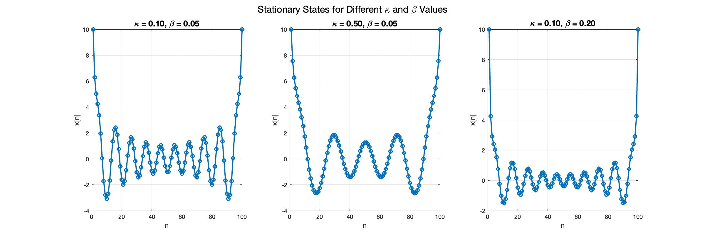
The solutions to this equation correspond to the various possible stable equilibrium states of the system, where each represents different static distribution patterns of displacements . The specific form of these stationary solutions depends on the system parameters, such as κ , ω, and β , as well as the initial and boundary conditions of the problem.
To find these solutions in a more specific form, one might need to solve the equation using analytical or numerical methods, considering the different cases that could arise in such a non-linear system.
By interpreting the equation in this way, we can relate the dynamics described by the discrete Klein - Gordon equation to the behavior of DNA molecules within a biological system . This analogy allows us to understand the behavior of DNA in terms of concepts from physics and mathematical modeling .
% Parameters
numBases = 100; % Number of spatial points
omegaD = 0.2; % Common parameter for the equation
% Preallocate the array for the function handles
equations = cell(numBases, 1);
% Initial guess for the solution
initialGuess = 0.01 * ones(numBases, 1);
% Parameter sets for kappa and beta
paramSets = [0.1, 0.05; 0.5, 0.05; 0.1, 0.2];
% Prepare figure for subplot
figure;
set(gcf, 'Position', [100, 100, 1200, 400]); % Set figure size
% Newton-Raphson method parameters
maxIterations = 1000;
tolerance = 1e-10;
% Set options for fsolve to use the 'levenberg-marquardt' algorithm
options = optimoptions('fsolve', 'Algorithm', 'levenberg-marquardt', 'MaxIterations', maxIterations, 'FunctionTolerance', tolerance);
for i = 1:size(paramSets, 1)
kappa = paramSets(i, 1);
beta = paramSets(i, 2);
% Define the equations using a function
for n = 2:numBases-1
equations{n} = @(x) -kappa * (x(n+1) - 2 * x(n) + x(n-1)) - omegaD^2 * (x(n) - beta * x(n)^3);
end
% Boundary conditions with specified fixed values
someFixedValue1 = 10; % Replace with actual value if needed
someFixedValue2 = 10; % Replace with actual value if needed
equations{1} = @(x) x(1) - someFixedValue1;
equations{numBases} = @(x) x(numBases) - someFixedValue2;
% Combine all equations into a single function
F = @(x) cell2mat(cellfun(@(f) f(x), equations, 'UniformOutput', false));
% Solve the system of equations using fsolve with the specified options
x_solution = fsolve(F, initialGuess, options);
norm(F(x_solution))
% Plot the solution in a subplot
subplot(1, 3, i);
plot(x_solution, 'o-', 'LineWidth', 2);
grid on;
xlabel('n', 'FontSize', 12);
ylabel('x[n]', 'FontSize', 12);
title(sprintf('\\kappa = %.2f, \\beta = %.2f', kappa, beta), 'FontSize', 14);
end
% Improve overall aesthetics
sgtitle('Stationary States for Different \kappa and \beta Values', 'FontSize', 16); % Super title for the figure
In the second plot, the elasticity constant κis increased to 0.5, representing a system with greater stiffness . This parameter influences how resistant the system is to deformation, implying that a higher κ makes the system more resilient to changes . By increasing κ, we are essentially tightening the interactions between adjacent units in the model, which could represent, for instance, stronger bonding forces in a physical or biological system .
In the third plot the nonlinearity coefficient β is increased to 0.2 . This adjustment enhances the nonlinear interactions within the system, which can lead to more complex dynamic behaviors, especially in systems exhibiting bifurcations or chaos under certain conditions .
The following expression
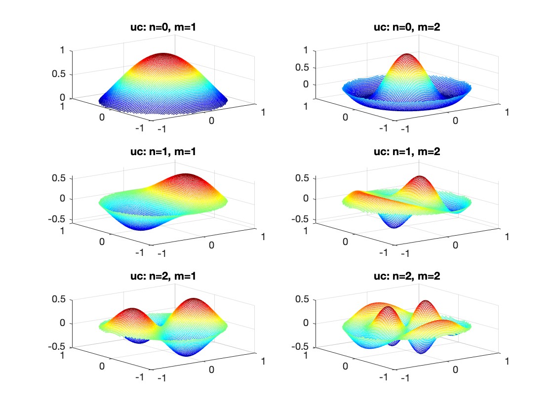
gives the solution for the Helmholtz problem. On the circular disc with center 0 and radius a. For the plot in 3-dimensional graphics of the solutions on Matlab for and then calculate some eigenfunctions with the following expression.
It could be better to separate functions with and as follows
diska = 1; % Radius of the disk
mmax = 2; % Maximum value of m
nmax = 2; % Maximum value of n
% Function to find the k-th zero of the n-th Bessel function
% This function uses a more accurate method for initial guess
besselzero = @(n, k) fzero(@(x) besselj(n, x), [(k-(n==0))*pi, (k+1-(n==0))*pi]);
% Define the eigenvalue k[m, n] based on the zeros of the Bessel function
k = @(m, n) besselzero(n, m);
% Define the functions uc and us using Bessel functions
% These functions represent the radial part of the solution
uc = @(r, t, m, n) cos(n * t) .* besselj(n, k(m, n) * r);
us = @(r, t, m, n) sin(n * t) .* besselj(n, k(m, n) * r);
% Generate data for demonstration
data = zeros(5, 3);
for m = 1:5
for n = 0:2
data(m, n+1) = k(m, n); % Storing the eigenvalues
end
end
% Display the data
disp(data);
% Plotting all in one figure
figure;
plotIndex = 1;
for n = 0:nmax
for m = 1:mmax
subplot(nmax + 1, mmax, plotIndex);
[X, Y] = meshgrid(linspace(-diska, diska, 100), linspace(-diska, diska, 100));
R = sqrt(X.^2 + Y.^2);
T = atan2(Y, X);
Z = uc(R, T, m, n); % Using uc for plotting
% Ensure the plot is only within the disk
Z(R > diska) = NaN;
mesh(X, Y, Z);
title(sprintf('uc: n=%d, m=%d', n, m));
colormap('jet');
plotIndex = plotIndex + 1;
end
end
First, I felt that the three answers provided by a user in this thread might have been generated by AI. How do you think?
Second, I found that "Responsible usage of generative AI tools, such as ChatGPT, is allowed in MATLAB Answers."
If the answers are indeed AI generated, then the user didn't do "clearly indicating when AI generated content is incorporated".
That leads to my question that how do we enforce the guideline.
I am not against using AI for answers but in this case, I felt the answering text is mentioning all the relevant words but missing the point. For novice users who are seeking answers, this would be misleading and waste of time.
Mathworks has always had quality documentation but in 2023, the documentation quality fell. Will this improve in 2024?
Hi
I have Matlab 2015b installed and if I try:
ones(2,3,4)+ones(2,3)
of course I get an error. But my student has R2023b installed and she gets a 2x3x4 matrix as a result, with all elements = 2.
How is it possible?
Thanks
A
This study explores the demographic patterns and disease outcomes during the cholera outbreak in London in 1849. Utilizing historical records and scholarly accounts, the research investigates the impact of the outbreak on the city' s population. While specific data for the 1849 cholera outbreak is limited, trends from similar 19th - century outbreaks suggest a high infection rate, potentially ranging from 30% to 50% of the population, owing to poor sanitation and overcrowded living conditions . Additionally, the birth rate in London during this period was estimated at 0.037 births per person per year . Although the exact reproduction number (R₀) for cholera in 1849 remains elusive, historical evidence implies a high R₀ due to the prevalent unsanitary conditions . This study sheds light on the challenges of estimating disease parameters from historical data, emphasizing the critical role of sanitation and public health measures in mitigating the impact of infectious diseases.
Introduction
The cholera outbreak of 1849 was a significant event in the history of cholera, a deadly waterborne disease caused by the bacterium Vibrio cholera. Cholera had several major outbreaks during the 19th century, and the one in 1849 was particularly devastating.
During this outbreak, cholera spread rapidly across Europe, including countries like England, France, and Germany . The disease also affected North America, with outbreaks reported in cities like New York and Montreal. The exact number of casualties from the 1849 cholera outbreak is difficult to determine due to limited record - keeping at that time. However, it is estimated that tens of thousands of people died as a result of the disease during this outbreak.
Cholera is highly contagious and spreads through contaminated water and food . The lack of proper sanitation and hygiene practices in the 19th century contributed to the rapid spread of the disease. It wasn't until the late 19th and early 20th centuries that advancements in public health, sanitation, and clean drinking water significantly reduced the incidence and impact of cholera outbreaks in many parts of the world.
Infection Rate
Based on general patterns observed in 19th - century cholera outbreaks and the conditions of that time, it' s reasonable to assume that the infection rate was quite high. During major cholera outbreaks in densely populated and unsanitary areas, infection rates could be as high as 30 - 50% or even more.
This means that in a densely populated city like London, with an estimated population of around 2.3 million in 1849, tens of thousands of people could have been infected during the outbreak. It' s important to emphasize that this is a rough estimation based on historical patterns and not specific to the 1849 outbreak. The actual infection rate could have varied widely based on the local conditions, public health measures in place, and the effectiveness of efforts to contain the disease.
For precise and localized estimations, detailed historical records specific to the 1849 cholera outbreak in a particular city or region would be required, and such data might not be readily available due to the limitations of historical documentation from that time period
Mortality Rate
It' s challenging to provide an exact death rate for the 1849 cholera outbreak because of the limited and often unreliable historical records from that time period. However, it is widely acknowledged that the death rate was significant, with tens of thousands of people dying as a result of the disease during this outbreak.
Cholera has historically been known for its high mortality rate, particularly in areas with poor sanitation and limited access to clean water. During cholera outbreaks in the 19th century, mortality rates could be extremely high, sometimes reaching 50% or more in affected communities. This high mortality rate was due to the rapid onset of severe dehydration and electrolyte imbalance caused by the cholera toxin, leading to death if not promptly treated.
Studies and historical accounts from various cholera outbreaks suggest that the R₀ for cholera can range from 1.5 to 2.5 or even higher in conditions where sanitation is inadequate and clean water is scarce. This means that one person with cholera could potentially infect 1.5 to 2.5 or more other people in such settings.
Unfortunately, there are no specific and reliable data available regarding the recovery rates from the 1849 cholera outbreak, as detailed and accurate record - keeping during that time period was limited. Cholera outbreaks in the 19th century were often devastating due to the lack of effective medical treatments and poor sanitation conditions. Recovery from cholera largely depended on the individual's ability to rehydrate, which was difficult given the rapid loss of fluids through severe diarrhea and vomiting .
LONDON CASE OF STUDY
In 1849, the estimated population of London was around 2.3 million people. London experienced significant population growth during the 19th century due to urbanization and industrialization. It’s important to note that historical population figures are often estimates, as comprehensive and accurate record-keeping methods were not as advanced as they are today.
% Define parameters
R0 = 2.5;
beta = 0.5;
gamma = 0.2; % Recovery rate
N = 2300000; % Total population
I0 = 1; % Initial number of infected individuals
% Define the SIR model differential equations
sir_eqns = @(t, Y) [-beta * Y(1) * Y(2) / N; % dS/dt
beta * Y(1) * Y(2) / N - gamma * Y(2); % dI/dt
gamma * Y(2)]; % dR/dt
% Initial conditions
Y0 = [N - I0; I0; 0]; % Initial conditions for S, I, R
% Time span
tmax1 = 100; % Define the maximum time (adjust as needed)
tspan = [0 tmax1];
% Solve the SIR model differential equations
[t, Y] = ode45(sir_eqns, tspan, Y0);
% Plot the results
figure;
plot(t, Y(:,1), 'b', t, Y(:,2), 'r', t, Y(:,3), 'g');
legend('Susceptible', 'Infected', 'Recovered');
xlabel('Time');
ylabel('Population');
title('SIR Model');
axis tight;
grid on;
% Assuming t and Y are obtained from the ode45 solver for the SIR model
% Extract the infected population data (second column of Y)
infected = Y(:,2);
% Plot the infected population over time
figure;
plot(t, infected, 'r');
legend('Infected');
xlabel('Time');
ylabel('Population');
title('Infected Population over Time');
grid on;
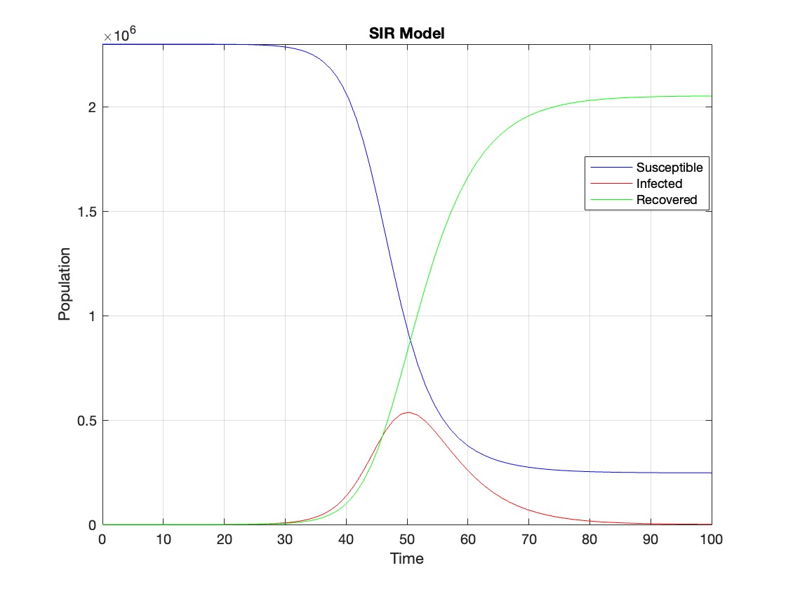
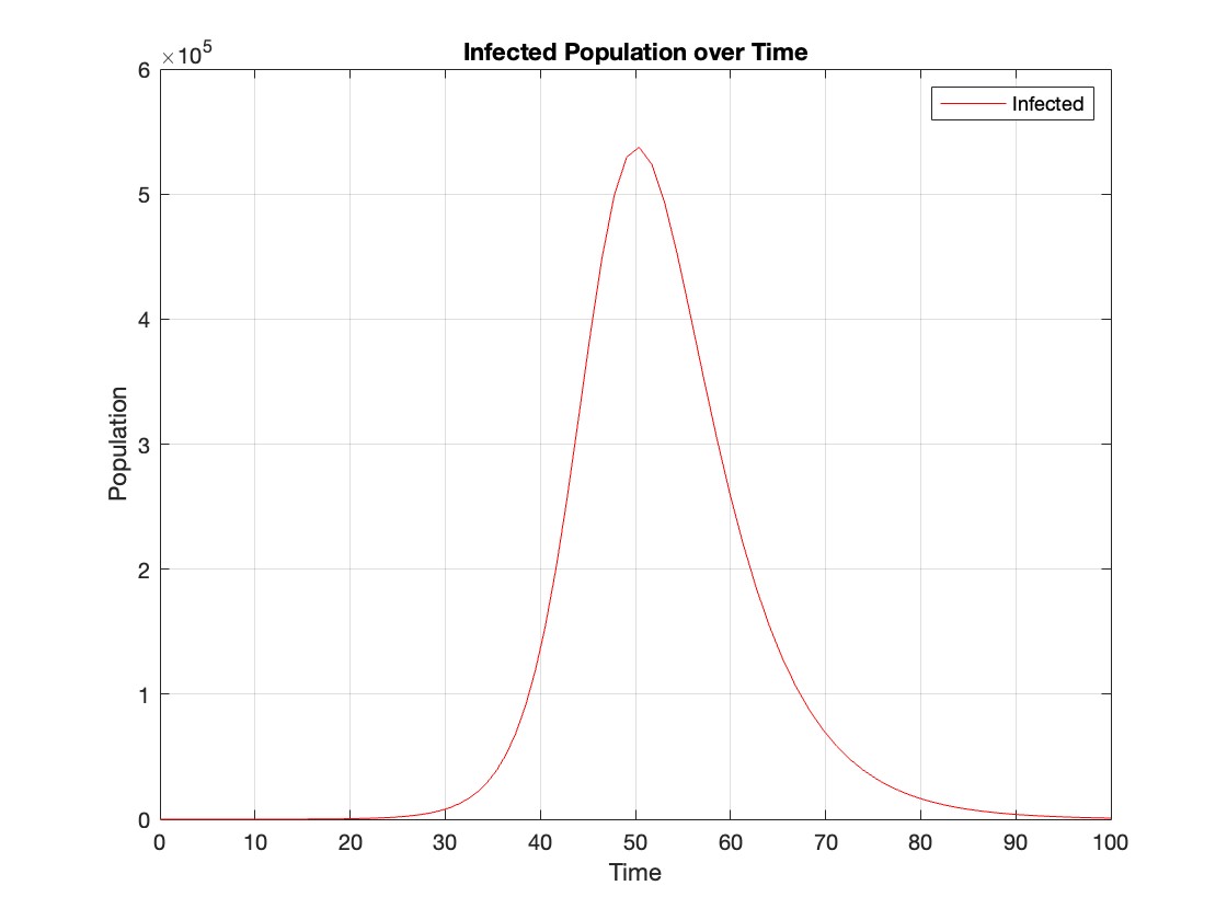
The code provides a visual representation of how the disease spreads and eventually diminishes within the population over the specified time interval . It can be used to understand the impact of different parameters (such as infection and recovery rates) on the progression of the outbreak .

The study of nonlinear dynamical systems in lattices is an area of research with continuously growing interest.The first systematic studies of these systems emerged in the late 1930 s,thanks to the work of Frenkel and Kontorova on crystal dislocations.These studies led to the formulation of the discrete Klein-Gordon equation (DKG).Specifically,in 1939,Frenkel and Kontorova proposed a model that describes the structure and dynamics of a crystal lattice in a dislocation core.The FK model has become one of the fundamental models in physics,as it has been proven to reliably describe significant phenomena observed in discrete media.The equation we will examine is a variation of the following form:
The process described involves approximating a nonlinear differential equation through the Taylor method and simplifying it into a linear model.Let's analyze step by step the process from the initial equation to its final form.For small angles, can be approximated through the Taylor series as:
We substitute in the original equation with the Taylor approximation:
To map this equation to a linear model,we consider the angles to correspond to displacements in a mass-spring system.Thus,the equation transforms into:
We recognize that the term expresses the nonlinearity of the system,while β is a coefficient corresponding to this nonlinearity,simplifying the expression.The final form of the equation is:
The exact value of β depends on the mapping of coefficients in the Taylor approximation and its application to the specific physical problem.Our main goal is to derive results regarding stability and convergence in nonlinear lattices under nonlinear conditions.We will examine the basic characteristics of the discrete Klein-Gordon equation:
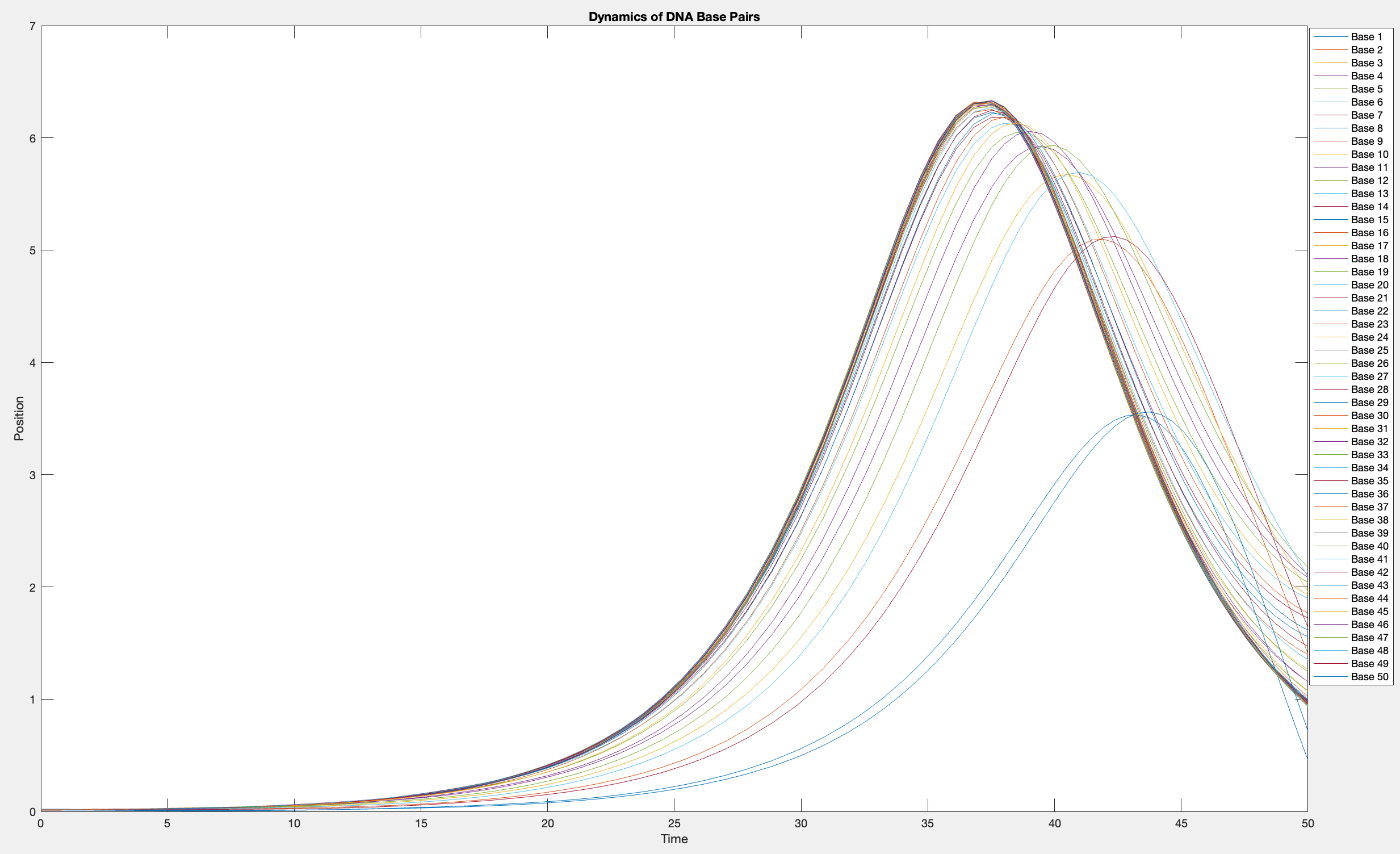
This model is often used to describe the opening of the DNA double helix during processes such as transcription.The model focuses on the transverse motion of the base pairs,which can be represented by a set of coupled nonlinear differential equations.
% Parameters
numBases = 50; % Number of base pairs
kappa = 0.1; % Elasticity constant
omegaD = 0.2; % Frequency term
beta = 0.05; % Nonlinearity coefficient
% Initial conditions
initialPositions = 0.01 + (0.02 - 0.01) * rand(numBases, 1);
initialVelocities = zeros(numBases, 1);
Time span
tSpan = [0 50];
>> % Differential equations
odeFunc = @(t, y) [y(numBases+1:end); ... % velocities
kappa * ([y(2); y(3:numBases); 0] - 2 * y(1:numBases) + [0; y(1:numBases-1)]) + ...
omegaD^2 * (y(1:numBases) - beta * y(1:numBases).^3)]; % accelerations
% Solve the system
[T, Y] = ode45(odeFunc, tSpan, [initialPositions; initialVelocities]);
% Visualization
plot(T, Y(:, 1:numBases))
legend(arrayfun(@(n) sprintf('Base %d', n), 1:numBases, 'UniformOutput', false))
xlabel('Time')
ylabel('Position')
title('Dynamics of DNA Base Pairs')
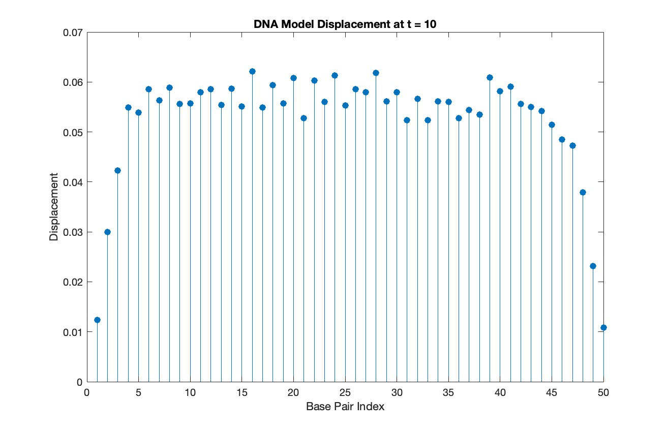
% Choose a specific time for the snapshot
snapshotTime = 10;
% Find the index in T that is closest to the snapshot time
[~, snapshotIndex] = min(abs(T - snapshotTime));
% Extract the solution at the snapshot time
snapshotSolution = Y(snapshotIndex, 1:numBases);
% Generate discrete plot for the DNA model at the snapshot time
figure;
stem(1:numBases, snapshotSolution, 'filled')
title(sprintf('DNA Model Displacement at t = %d', snapshotTime))
xlabel('Base Pair Index')
ylabel('Displacement')
% Time vector for detailed sampling
tDetailed = 0:0.5:50;
% Initialize an empty array to hold the data
data = [];
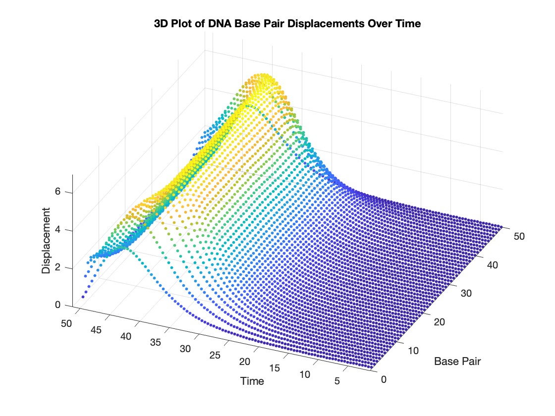
% Generate the data for 3D plotting
for i = 1:numBases
% Interpolate to get detailed solution data for each base pair
detailedSolution = interp1(T, Y(:, i), tDetailed);
% Concatenate the current base pair's data to the main data array
data = [data; repmat(i, length(tDetailed), 1), tDetailed', detailedSolution'];
end
% 3D Plot
figure;
scatter3(data(:,1), data(:,2), data(:,3), 10, data(:,3), 'filled')
xlabel('Base Pair')
ylabel('Time')
zlabel('Displacement')
title('3D Plot of DNA Base Pair Displacements Over Time')
colormap('rainbow')
colorbar