Risultati per
I am deeply honored to announce the official publication of my latest academic volume:
MATLAB for Civil Engineers: From Basics to Advanced Applications
(Springer Nature, 2025).
This work serves as a comprehensive bridge between theoretical civil engineering principles and their practical implementation through MATLAB—a platform essential to the future of computational design, simulation, and optimization in our field.
Structured to serve both academic audiences and practicing engineers, this book progresses from foundational MATLAB programming concepts to highly specialized applications in structural analysis, geotechnical engineering, hydraulic modeling, and finite element methods. Whether you are a student building analytical fluency or a professional seeking computational precision, this volume offers an indispensable resource for mastering MATLAB's full potential in civil engineering contexts.
With rigorously structured examples, case studies, and research-aligned methods, MATLAB for Civil Engineers reflects the convergence of engineering logic with algorithmic innovation—equipping readers to address contemporary challenges with clarity, accuracy, and foresight.
📖 Ideal for:
— Graduate and postgraduate civil engineering students
— University instructors and lecturers seeking a structured teaching companion
— Professionals aiming to integrate MATLAB into complex real-world projects
If you are passionate about engineering resilience, data-informed design, or computational modeling, I invite you to explore the work and share it with your network.
🧠 Let us advance the discipline together through precision, programming, and purpose.

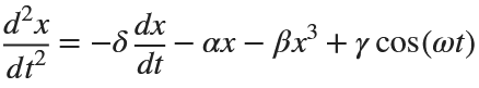
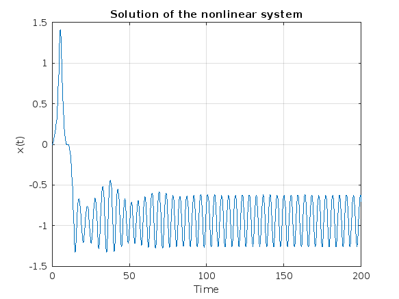
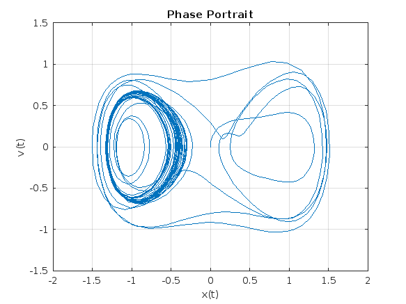
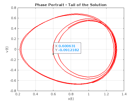
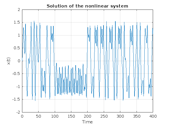
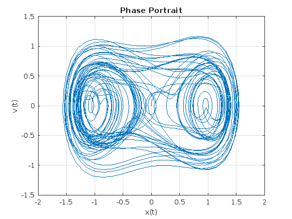
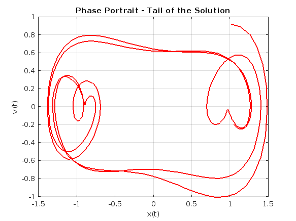
Following on from my previous post The Non-Chaotic Duffing Equation, now we will study the chaotic behaviour of the Duffing Equation
P.s:Any comments/advice on improving the code is welcome.
The Original Duffing Equation is the following:
Let 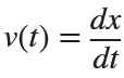 . This implies that
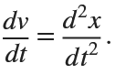
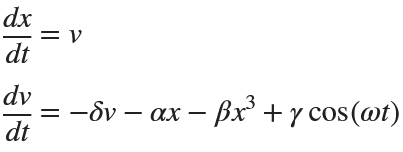
Then we rewrite it as a System of First-Order Equations
Using the substitution  for
for  , the second-order equation can be transformed into the following system of first-order equations:
Exploring the Effect of γ.
% Define parameters
gamma = 0.1;
alpha = -1;
beta = 1;
delta = 0.1;
omega = 1.4;
% Define the system of equations
odeSystem = @(t, y) [y(2);
-delta*y(2) - alpha*y(1) - beta*y(1)^3 + gamma*cos(omega*t)];
% Initial conditions
y0 = [0; 0]; % x(0) = 0, v(0) = 0
% Time span
tspan = [0 200];
% Solve the system
[t, y] = ode45(odeSystem, tspan, y0);
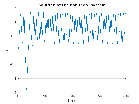
% Plot the results
figure;
plot(t, y(:, 1));
xlabel('Time');
ylabel('x(t)');
title('Solution of the nonlinear system');
grid on;
% Plot the phase portrait
figure;
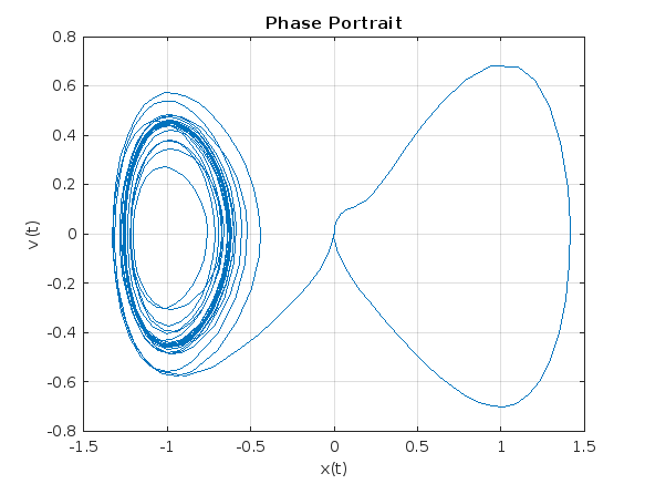
plot(y(:, 1), y(:, 2));
xlabel('x(t)');
ylabel('v(t)');
title('Phase Portrait');
grid on;
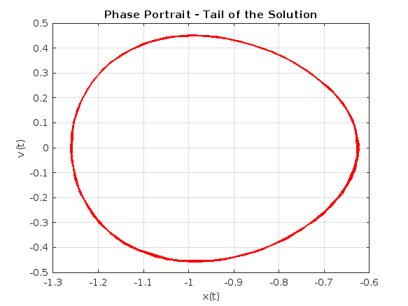
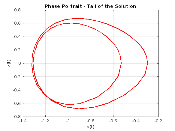
% Define the tail (e.g., last 10% of the time interval)
tail_start = floor(0.9 * length(t)); % Starting index for the tail
tail_end = length(t); % Ending index for the tail
% Plot the tail of the solution
figure;
plot(y(tail_start:tail_end, 1), y(tail_start:tail_end, 2), 'r', 'LineWidth', 1.5);
xlabel('x(t)');
ylabel('v(t)');
title('Phase Portrait - Tail of the Solution');
grid on;
% Define parameters
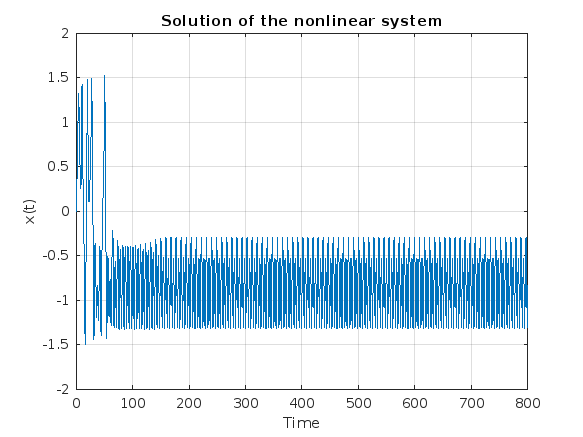
gamma = 0.318;
alpha = -1;
beta = 1;
delta = 0.1;
omega = 1.4;
% Define the system of equations
odeSystem = @(t, y) [y(2);
-delta*y(2) - alpha*y(1) - beta*y(1)^3 + gamma*cos(omega*t)];
% Initial conditions
y0 = [0; 0]; % x(0) = 0, v(0) = 0
% Time span
tspan = [0 800];
% Solve the system
[t, y] = ode45(odeSystem, tspan, y0);
% Plot the results
figure;
plot(t, y(:, 1));
xlabel('Time');
ylabel('x(t)');
title('Solution of the nonlinear system');
grid on;
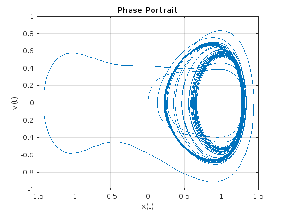
% Plot the phase portrait
figure;
plot(y(:, 1), y(:, 2));
xlabel('x(t)');
ylabel('v(t)');
title('Phase Portrait');
grid on;
% Define the tail (e.g., last 10% of the time interval)
tail_start = floor(0.9 * length(t)); % Starting index for the tail
tail_end = length(t); % Ending index for the tail
% Plot the tail of the solution
figure;
plot(y(tail_start:tail_end, 1), y(tail_start:tail_end, 2), 'r', 'LineWidth', 1.5);
xlabel('x(t)');
ylabel('v(t)');
title('Phase Portrait - Tail of the Solution');
grid on;
% Define parameters
gamma = 0.338;
alpha = -1;
beta = 1;
delta = 0.1;
omega = 1.4;
% Define the system of equations
odeSystem = @(t, y) [y(2);
-delta*y(2) - alpha*y(1) - beta*y(1)^3 + gamma*cos(omega*t)];
% Initial conditions
y0 = [0; 0]; % x(0) = 0, v(0) = 0
% Time span with more points for better resolution
tspan = linspace(0, 200,2000); % Increase the number of points
% Solve the system
[t, y] = ode45(odeSystem, tspan, y0);
% Plot the results
figure;
plot(t, y(:, 1));
xlabel('Time');
ylabel('x(t)');
title('Solution of the nonlinear system');
grid on;
% Plot the phase portrait
figure;
plot(y(:, 1), y(:, 2));
xlabel('x(t)');
ylabel('v(t)');
title('Phase Portrait');
grid on;
% Define the tail (e.g., last 10% of the time interval)
tail_start = floor(0.9 * length(t)); % Starting index for the tail
tail_end = length(t); % Ending index for the tail
% Plot the tail of the solution
figure;
plot(y(tail_start:tail_end, 1), y(tail_start:tail_end, 2), 'r', 'LineWidth', 1.5);
xlabel('x(t)');
ylabel('v(t)');
title('Phase Portrait - Tail of the Solution');
grid on;
ax = gca;
chart = ax.Children(1);
datatip(chart,0.5581,-0.1126);
% Define parameters
gamma = 0.35;
alpha = -1;
beta = 1;
delta = 0.1;
omega = 1.4;
% Define the system of equations
odeSystem = @(t, y) [y(2);
-delta*y(2) - alpha*y(1) - beta*y(1)^3 + gamma*cos(omega*t)];
% Initial conditions
y0 = [0; 0]; % x(0) = 0, v(0) = 0
% Time span with more points for better resolution
tspan = linspace(0, 400,3000); % Increase the number of points
% Solve the system
[t, y] = ode45(odeSystem, tspan, y0);
% Plot the results
figure;
plot(t, y(:, 1));
xlabel('Time');
ylabel('x(t)');
title('Solution of the nonlinear system');
grid on;
% Plot the phase portrait
figure;
plot(y(:, 1), y(:, 2));
xlabel('x(t)');
ylabel('v(t)');
title('Phase Portrait');
grid on;
% Define the tail (e.g., last 10% of the time interval)
tail_start = floor(0.9 * length(t)); % Starting index for the tail
tail_end = length(t); % Ending index for the tail
% Plot the tail of the solution
figure;
plot(y(tail_start:tail_end, 1), y(tail_start:tail_end, 2), 'r', 'LineWidth', 1.5);
xlabel('x(t)');
ylabel('v(t)');
title('Phase Portrait - Tail of the Solution');
grid on;
Studying the attached document Duffing Equation from the University of Colorado, I noticed that there is an analysis of The Non-Chaotic Duffing Equation and all the graphs were created with Matlab. And since the code is not given I took the initiative to try to create the same graphs with the following code.
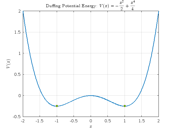
- Plotting the Potential Energy and Identifying Extrema
% Define the range of x values
x = linspace(-2, 2, 1000);
% Define the potential function V(x)
V = -x.^2 / 2 + x.^4 / 4;
% Plot the potential function
figure;
plot(x, V, 'LineWidth', 2);
hold on;
% Mark the minima at x = ±1
plot([-1, 1], [-1/4, -1/4], 'ro', 'MarkerSize', 5, 'MarkerFaceColor', 'g');
% Add LaTeX title and labels
title('Duffing Potential Energy: $$V(x) = -\frac{x^2}{2} + \frac{x^4}{4}$$', 'Interpreter', 'latex');
xlabel('$$x$$', 'Interpreter', 'latex');
ylabel('$$V(x)$$','Interpreter', 'latex');
grid on;
hold off;
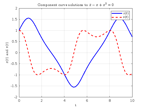
- Solving and Plotting the Duffing Equation
% Define the system of ODEs for the non-chaotic Duffing equation
duffing_ode = @(t, X) [X(2);
X(1) - X(1).^3];
% Time span for the simulation
tspan = [0 10];
% Initial conditions [x(0), v(0)]
initial_conditions = [1; 1];
% Solve the ODE using ode45
[t, X] = ode45(duffing_ode, tspan, initial_conditions);
% Extract displacement (x) and velocity (v)
x = X(:, 1);
v = X(:, 2);
% Plot both x(t) and v(t) in the same figure
figure;
plot(t, x, 'b-', 'LineWidth', 2); % Plot x(t) with blue line
hold on;
plot(t, v, 'r--', 'LineWidth', 2); % Plot v(t) with red dashed line
% Add title, labels, and legend
title(' Component curve solutions to $$\ddot{x}-x+x^3=0$$','Interpreter', 'latex');
xlabel('t','Interpreter', 'latex');
ylabel('$$x(t) $$ and $$v(t) $$','Interpreter', 'latex');
legend('$$x(t)$$', ' $$v(t)$$','Interpreter', 'latex');
grid on;
hold off;
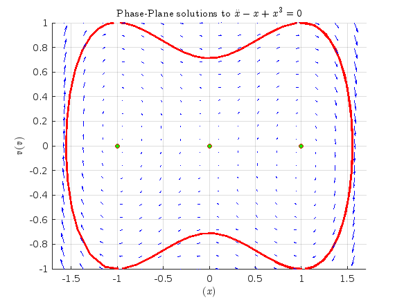
% Phase portrait with nullclines, equilibria, and vector field
figure;
hold on;
% Plot phase portrait
plot(x, v,'r', 'LineWidth', 2);
% Plot equilibrium points
plot([0 1 -1], [0 0 0], 'ro', 'MarkerSize', 5, 'MarkerFaceColor', 'g');
% Create a grid of points for the vector field
[x_vals, v_vals] = meshgrid(linspace(-2, 2, 20), linspace(-1, 1, 20));
% Compute the vector field components
dxdt = v_vals;
dvdt = x_vals - x_vals.^3;
% Plot the vector field
quiver(x_vals, v_vals, dxdt, dvdt, 'b');
% Set axis limits to [-1, 1]
xlim([-1.7 1.7]);
ylim([-1 1]);
% Labels and title
title('Phase-Plane solutions to $$\ddot{x}-x+x^3=0$$','Interpreter', 'latex');
xlabel('$$ (x)$$','Interpreter', 'latex');
ylabel('$$v(v)$$','Interpreter', 'latex');
grid on;
hold off;
The study of the dynamics of the discrete Klein - Gordon equation (DKG) with friction is given by the equation :

above equation, W describes the potential function :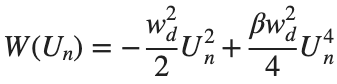
The objective of this simulation is to model the dynamics of a segment of DNA under thermal fluctuations with fixed boundaries using a modified discrete Klein-Gordon equation. The model incorporates elasticity, nonlinearity, and damping to provide insights into the mechanical behavior of DNA under various conditions.
% Parameters
numBases = 200; % Number of base pairs, representing a segment of DNA
kappa = 0.1; % Elasticity constant
omegaD = 0.2; % Frequency term
beta = 0.05; % Nonlinearity coefficient
delta = 0.01; % Damping coefficient
- Position: Random initial perturbations between 0.01 and 0.02 to simulate the thermal fluctuations at the start.
- Velocity: All bases start from rest, assuming no initial movement except for the thermal perturbations.
% Random initial perturbations to simulate thermal fluctuations
initialPositions = 0.01 + (0.02-0.01).*rand(numBases,1);
initialVelocities = zeros(numBases,1); % Assuming initial rest state
The simulation uses fixed ends to model the DNA segment being anchored at both ends, which is typical in experimental setups for studying DNA mechanics. The equations of motion for each base are derived from a modified discrete Klein-Gordon equation with the inclusion of damping:
% Define the differential equations
dt = 0.05; % Time step
tmax = 50; % Maximum time
tspan = 0:dt:tmax; % Time vector
x = zeros(numBases, length(tspan)); % Displacement matrix
x(:,1) = initialPositions; % Initial positions
% Velocity-Verlet algorithm for numerical integration
for i = 2:length(tspan)
% Compute acceleration for internal bases
acceleration = zeros(numBases,1);
for n = 2:numBases-1
acceleration(n) = kappa * (x(n+1, i-1) - 2 * x(n, i-1) + x(n-1, i-1)) ...
- delta * initialVelocities(n) - omegaD^2 * (x(n, i-1) - beta * x(n, i-1)^3);
end
% positions for internal bases
x(2:numBases-1, i) = x(2:numBases-1, i-1) + dt * initialVelocities(2:numBases-1) ...
+ 0.5 * dt^2 * acceleration(2:numBases-1);
% velocities using new accelerations
newAcceleration = zeros(numBases,1);
for n = 2:numBases-1
newAcceleration(n) = kappa * (x(n+1, i) - 2 * x(n, i) + x(n-1, i)) ...
- delta * initialVelocities(n) - omegaD^2 * (x(n, i) - beta * x(n, i)^3);
end
initialVelocities(2:numBases-1) = initialVelocities(2:numBases-1) + 0.5 * dt * (acceleration(2:numBases-1) + newAcceleration(2:numBases-1));
end
% Visualization of displacement over time for each base pair
figure;
hold on;
for n = 2:numBases-1
plot(tspan, x(n, :));
end
xlabel('Time');
ylabel('Displacement');
legend(arrayfun(@(n) ['Base ' num2str(n)], 2:numBases-1, 'UniformOutput', false));
title('Displacement of DNA Bases Over Time');
hold off;
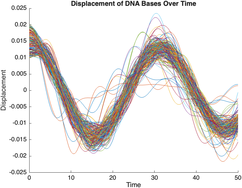
The results are visualized using a plot that shows the displacements of each base over time . Key observations from the simulation include :
- Wave Propagation: The initial perturbations lead to wave-like dynamics along the segment, with visible propagation and reflection at the boundaries.
- Damping Effects: The inclusion of damping leads to a gradual reduction in the amplitude of the oscillations, indicating energy dissipation over time.
- Nonlinear Behavior: The nonlinear term influences the response, potentially stabilizing the system against large displacements or leading to complex dynamic patterns.
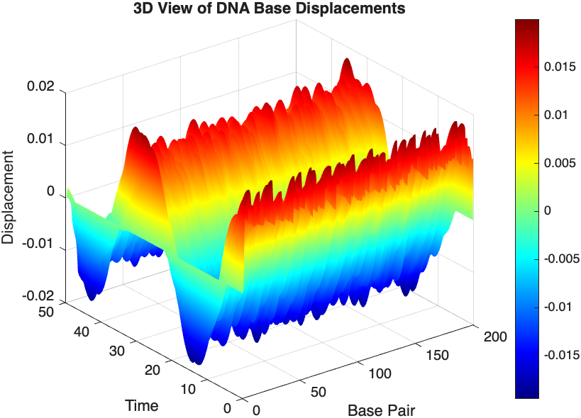
% 3D plot for displacement
figure;
[X, T] = meshgrid(1:numBases, tspan);
surf(X', T', x);
xlabel('Base Pair');
ylabel('Time');
zlabel('Displacement');
title('3D View of DNA Base Displacements');
colormap('jet');
shading interp;
colorbar; % Adds a color bar to indicate displacement magnitude
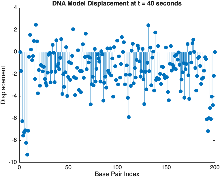
% Snapshot visualization at a specific time
snapshotTime = 40; % Desired time for the snapshot
[~, snapshotIndex] = min(abs(tspan - snapshotTime)); % Find closest index
snapshotSolution = x(:, snapshotIndex); % Extract displacement at the snapshot time
% Plotting the snapshot
figure;
stem(1:numBases, snapshotSolution, 'filled'); % Discrete plot using stem
title(sprintf('DNA Model Displacement at t = %d seconds', snapshotTime));
xlabel('Base Pair Index');
ylabel('Displacement');
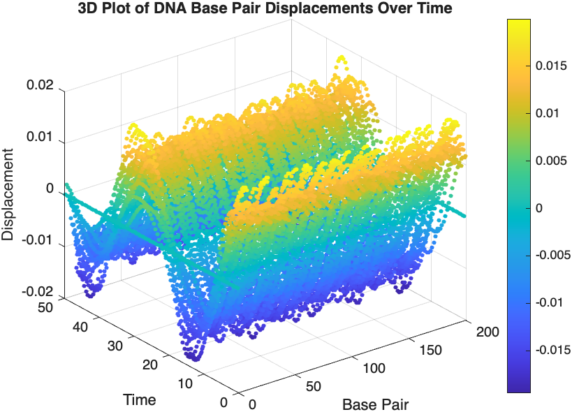
% Time vector for detailed sampling
tDetailed = 0:0.5:50; % Detailed time steps
% Initialize an empty array to hold the data
data = [];
% Generate the data for 3D plotting
for i = 1:numBases
% Interpolate to get detailed solution data for each base pair
detailedSolution = interp1(tspan, x(i, :), tDetailed);
% Concatenate the current base pair's data to the main data array
data = [data; repmat(i, length(tDetailed), 1), tDetailed', detailedSolution'];
end
% 3D Plot
figure;
scatter3(data(:,1), data(:,2), data(:,3), 10, data(:,3), 'filled');
xlabel('Base Pair');
ylabel('Time');
zlabel('Displacement');
title('3D Plot of DNA Base Pair Displacements Over Time');
colorbar; % Adds a color bar to indicate displacement magnitude
Before we begin, you will need to make sure you have 'sir_age_model.m' installed. Once you've downloaded this folder into your working directory, which can be located at your current folder. If you can see this file in your current folder, then it's safe to use it. If you choose to use MATLAB online or MATLAB Mobile, you may upload this to your MATLAB Drive.
This is the code for the SIR model stratified into 2 age groups (children and adults). For a detailed explanation of how to derive the force of infection by age group.
% Main script to run the SIR model simulation
% Initial state values
initial_state_values = [200000; 1; 0; 800000; 0; 0]; % [S1; I1; R1; S2; I2; R2]
% Parameters
parameters = [0.05; 7; 6; 1; 10; 1/5]; % [b; c_11; c_12; c_21; c_22; gamma]
% Time span for the simulation (3 months, with daily steps)
tspan = [0 90];
% Solve the ODE
[t, y] = ode45(@(t, y) sir_age_model(t, y, parameters), tspan, initial_state_values);
% Plotting the results
plot(t, y);
xlabel('Time (days)');
ylabel('Number of people');
legend('S1', 'I1', 'R1', 'S2', 'I2', 'R2');
title('SIR Model with Age Structure');
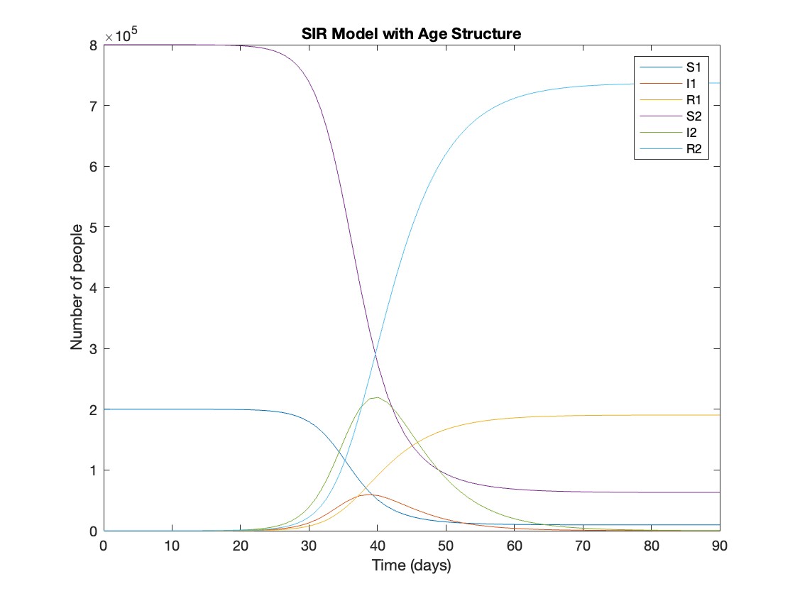
What was the cumulative incidence of infection during this epidemic? What proportion of those infections occurred in children?
In the SIR model, the cumulative incidence of infection is simply the decline in susceptibility.
% Assuming 'y' contains the simulation results from the ode45 function
% and 't' contains the time points
% Total cumulative incidence
total_cumulative_incidence = (y(1,1) - y(end,1)) + (y(1,4) - y(end,4));
fprintf('Total cumulative incidence: %f\n', total_cumulative_incidence);
% Cumulative incidence in children
cumulative_incidence_children = (y(1,1) - y(end,1));
% Proportion of infections in children
proportion_infections_children = cumulative_incidence_children / total_cumulative_incidence;
fprintf('Proportion of infections in children: %f\n', proportion_infections_children);
927,447 people became infected during this epidemic, 20.5% of which were children.
Which age group was most affected by the epidemic?
To answer this, we can calculate the proportion of children and adults that became infected.
% Assuming 'y' contains the simulation results from the ode45 function
% and 't' contains the time points
% Proportion of children that became infected
initial_children = 200000; % initial number of susceptible children
final_susceptible_children = y(end,1); % final number of susceptible children
proportion_infected_children = (initial_children - final_susceptible_children) / initial_children;
fprintf('Proportion of children that became infected: %f\n', proportion_infected_children);
% Proportion of adults that became infected
initial_adults = 800000; % initial number of susceptible adults
final_susceptible_adults = y(end,4); % final number of susceptible adults
proportion_infected_adults = (initial_adults - final_susceptible_adults) / initial_adults;
fprintf('Proportion of adults that became infected: %f\n', proportion_infected_adults);
Throughout this epidemic, 95% of all children and 92% of all adults were infected. Children were therefore slightly more affected in proportion to their population size, even though the majority of infections occurred in adults.
This study explores the demographic patterns and disease outcomes during the cholera outbreak in London in 1849. Utilizing historical records and scholarly accounts, the research investigates the impact of the outbreak on the city' s population. While specific data for the 1849 cholera outbreak is limited, trends from similar 19th - century outbreaks suggest a high infection rate, potentially ranging from 30% to 50% of the population, owing to poor sanitation and overcrowded living conditions . Additionally, the birth rate in London during this period was estimated at 0.037 births per person per year . Although the exact reproduction number (R₀) for cholera in 1849 remains elusive, historical evidence implies a high R₀ due to the prevalent unsanitary conditions . This study sheds light on the challenges of estimating disease parameters from historical data, emphasizing the critical role of sanitation and public health measures in mitigating the impact of infectious diseases.
Introduction
The cholera outbreak of 1849 was a significant event in the history of cholera, a deadly waterborne disease caused by the bacterium Vibrio cholera. Cholera had several major outbreaks during the 19th century, and the one in 1849 was particularly devastating.
During this outbreak, cholera spread rapidly across Europe, including countries like England, France, and Germany . The disease also affected North America, with outbreaks reported in cities like New York and Montreal. The exact number of casualties from the 1849 cholera outbreak is difficult to determine due to limited record - keeping at that time. However, it is estimated that tens of thousands of people died as a result of the disease during this outbreak.
Cholera is highly contagious and spreads through contaminated water and food . The lack of proper sanitation and hygiene practices in the 19th century contributed to the rapid spread of the disease. It wasn't until the late 19th and early 20th centuries that advancements in public health, sanitation, and clean drinking water significantly reduced the incidence and impact of cholera outbreaks in many parts of the world.
Infection Rate
Based on general patterns observed in 19th - century cholera outbreaks and the conditions of that time, it' s reasonable to assume that the infection rate was quite high. During major cholera outbreaks in densely populated and unsanitary areas, infection rates could be as high as 30 - 50% or even more.
This means that in a densely populated city like London, with an estimated population of around 2.3 million in 1849, tens of thousands of people could have been infected during the outbreak. It' s important to emphasize that this is a rough estimation based on historical patterns and not specific to the 1849 outbreak. The actual infection rate could have varied widely based on the local conditions, public health measures in place, and the effectiveness of efforts to contain the disease.
For precise and localized estimations, detailed historical records specific to the 1849 cholera outbreak in a particular city or region would be required, and such data might not be readily available due to the limitations of historical documentation from that time period
Mortality Rate
It' s challenging to provide an exact death rate for the 1849 cholera outbreak because of the limited and often unreliable historical records from that time period. However, it is widely acknowledged that the death rate was significant, with tens of thousands of people dying as a result of the disease during this outbreak.
Cholera has historically been known for its high mortality rate, particularly in areas with poor sanitation and limited access to clean water. During cholera outbreaks in the 19th century, mortality rates could be extremely high, sometimes reaching 50% or more in affected communities. This high mortality rate was due to the rapid onset of severe dehydration and electrolyte imbalance caused by the cholera toxin, leading to death if not promptly treated.
Studies and historical accounts from various cholera outbreaks suggest that the R₀ for cholera can range from 1.5 to 2.5 or even higher in conditions where sanitation is inadequate and clean water is scarce. This means that one person with cholera could potentially infect 1.5 to 2.5 or more other people in such settings.
Unfortunately, there are no specific and reliable data available regarding the recovery rates from the 1849 cholera outbreak, as detailed and accurate record - keeping during that time period was limited. Cholera outbreaks in the 19th century were often devastating due to the lack of effective medical treatments and poor sanitation conditions. Recovery from cholera largely depended on the individual's ability to rehydrate, which was difficult given the rapid loss of fluids through severe diarrhea and vomiting .
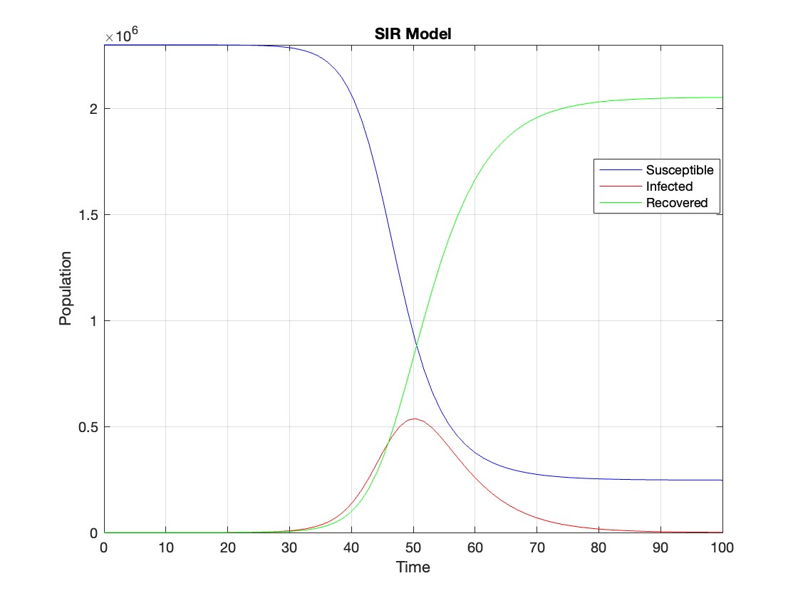
LONDON CASE OF STUDY
In 1849, the estimated population of London was around 2.3 million people. London experienced significant population growth during the 19th century due to urbanization and industrialization. It’s important to note that historical population figures are often estimates, as comprehensive and accurate record-keeping methods were not as advanced as they are today.
% Define parameters
R0 = 2.5;
beta = 0.5;
gamma = 0.2; % Recovery rate
N = 2300000; % Total population
I0 = 1; % Initial number of infected individuals
% Define the SIR model differential equations
sir_eqns = @(t, Y) [-beta * Y(1) * Y(2) / N; % dS/dt
beta * Y(1) * Y(2) / N - gamma * Y(2); % dI/dt
gamma * Y(2)]; % dR/dt
% Initial conditions
Y0 = [N - I0; I0; 0]; % Initial conditions for S, I, R
% Time span
tmax1 = 100; % Define the maximum time (adjust as needed)
tspan = [0 tmax1];
% Solve the SIR model differential equations
[t, Y] = ode45(sir_eqns, tspan, Y0);
% Plot the results
figure;
plot(t, Y(:,1), 'b', t, Y(:,2), 'r', t, Y(:,3), 'g');
legend('Susceptible', 'Infected', 'Recovered');
xlabel('Time');
ylabel('Population');
title('SIR Model');
axis tight;
grid on;
% Assuming t and Y are obtained from the ode45 solver for the SIR model
% Extract the infected population data (second column of Y)
infected = Y(:,2);
% Plot the infected population over time
figure;
plot(t, infected, 'r');
legend('Infected');
xlabel('Time');
ylabel('Population');
title('Infected Population over Time');
grid on;
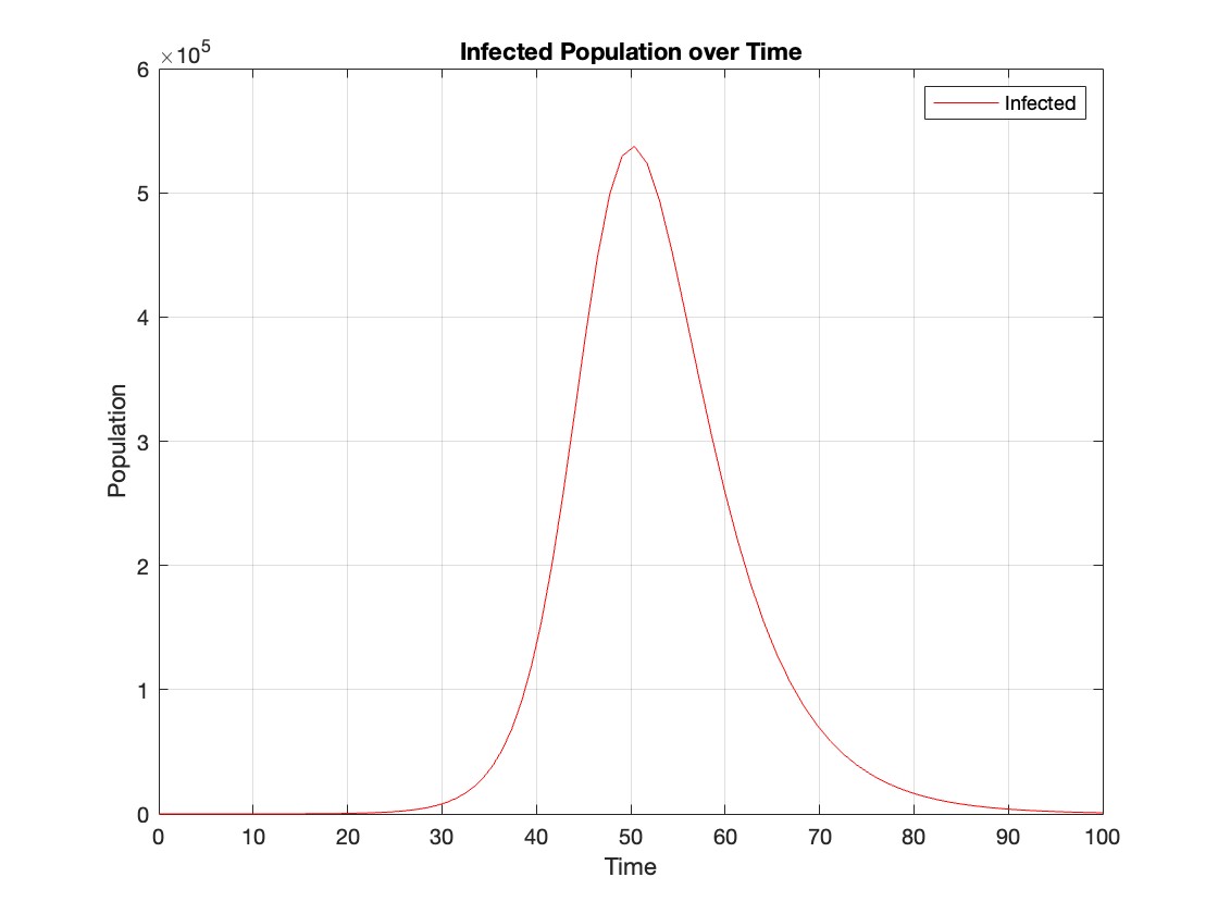
The code provides a visual representation of how the disease spreads and eventually diminishes within the population over the specified time interval . It can be used to understand the impact of different parameters (such as infection and recovery rates) on the progression of the outbreak .
The study of nonlinear dynamical systems in lattices is an area of research with continuously growing interest.The first systematic studies of these systems emerged in the late 1930 s,thanks to the work of Frenkel and Kontorova on crystal dislocations.These studies led to the formulation of the discrete Klein-Gordon equation (DKG).Specifically,in 1939,Frenkel and Kontorova proposed a model that describes the structure and dynamics of a crystal lattice in a dislocation core.The FK model has become one of the fundamental models in physics,as it has been proven to reliably describe significant phenomena observed in discrete media.The equation we will examine is a variation of the following form:

The process described involves approximating a nonlinear differential equation through the Taylor method and simplifying it into a linear model.Let's analyze step by step the process from the initial equation to its final form.For small angles, can be approximated through the Taylor series as:
We substitute  in the original equation with the Taylor approximation:
To map this equation to a linear model,we consider the angles  to correspond to displacements
  in a mass-spring system.Thus,the equation transforms into:
to correspond to displacements We recognize that the term  expresses the nonlinearity of the system,while β is a coefficient corresponding to this nonlinearity,simplifying the expression.The final form of the equation is:
The exact value of β depends on the mapping of coefficients in the Taylor approximation and its application to the specific physical problem.Our main goal is to derive results regarding stability and convergence in nonlinear lattices under nonlinear conditions.We will examine the basic characteristics of the discrete Klein-Gordon equation:
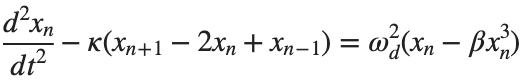
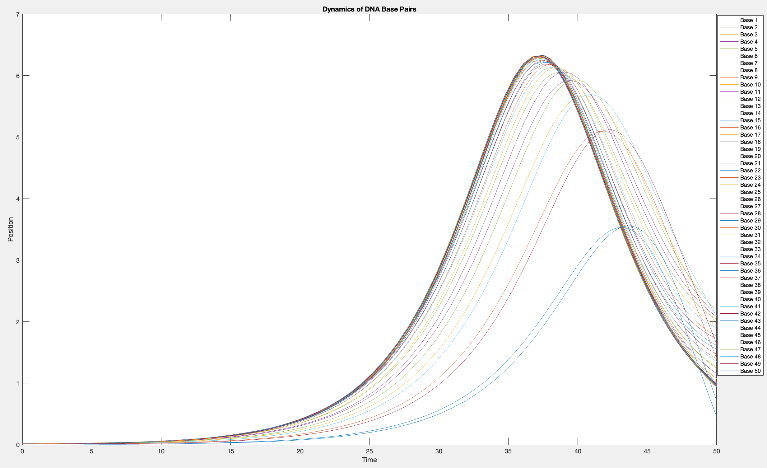
This model is often used to describe the opening of the DNA double helix during processes such as transcription.The model focuses on the transverse motion of the base pairs,which can be represented by a set of coupled nonlinear differential equations.
% Parameters
numBases = 50; % Number of base pairs
kappa = 0.1; % Elasticity constant
omegaD = 0.2; % Frequency term
beta = 0.05; % Nonlinearity coefficient
% Initial conditions
initialPositions = 0.01 + (0.02 - 0.01) * rand(numBases, 1);
initialVelocities = zeros(numBases, 1);
Time span
tSpan = [0 50];
>> % Differential equations
odeFunc = @(t, y) [y(numBases+1:end); ... % velocities
kappa * ([y(2); y(3:numBases); 0] - 2 * y(1:numBases) + [0; y(1:numBases-1)]) + ...
omegaD^2 * (y(1:numBases) - beta * y(1:numBases).^3)]; % accelerations
% Solve the system
[T, Y] = ode45(odeFunc, tSpan, [initialPositions; initialVelocities]);
% Visualization
plot(T, Y(:, 1:numBases))
legend(arrayfun(@(n) sprintf('Base %d', n), 1:numBases, 'UniformOutput', false))
xlabel('Time')
ylabel('Position')
title('Dynamics of DNA Base Pairs')
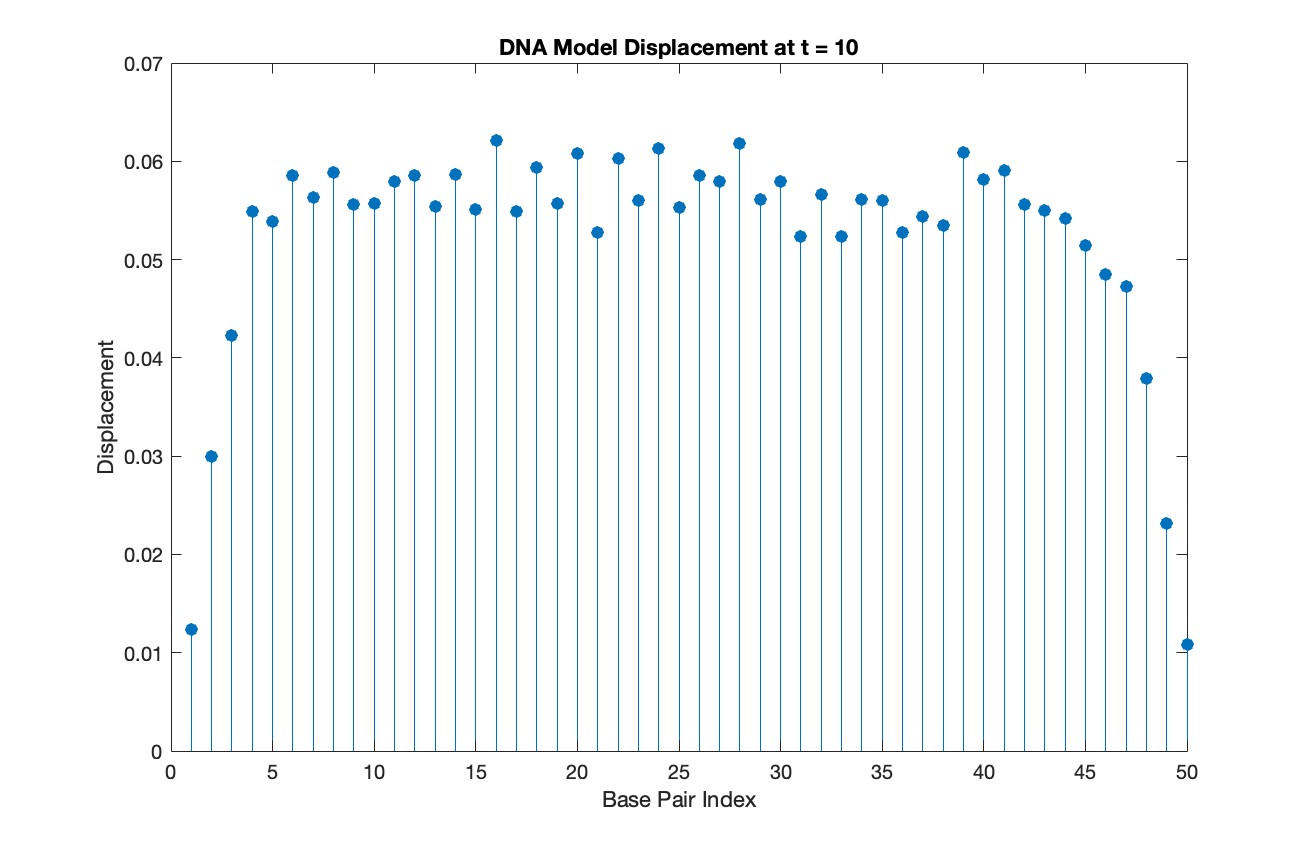
% Choose a specific time for the snapshot
snapshotTime = 10;
% Find the index in T that is closest to the snapshot time
[~, snapshotIndex] = min(abs(T - snapshotTime));
% Extract the solution at the snapshot time
snapshotSolution = Y(snapshotIndex, 1:numBases);
% Generate discrete plot for the DNA model at the snapshot time
figure;
stem(1:numBases, snapshotSolution, 'filled')
title(sprintf('DNA Model Displacement at t = %d', snapshotTime))
xlabel('Base Pair Index')
ylabel('Displacement')
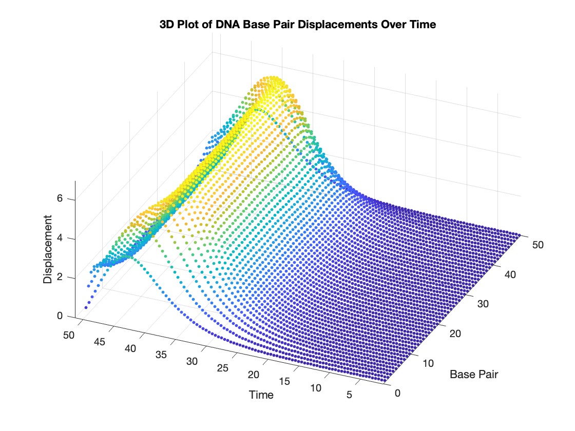
% Time vector for detailed sampling
tDetailed = 0:0.5:50;
% Initialize an empty array to hold the data
data = [];
% Generate the data for 3D plotting
for i = 1:numBases
% Interpolate to get detailed solution data for each base pair
detailedSolution = interp1(T, Y(:, i), tDetailed);
% Concatenate the current base pair's data to the main data array
data = [data; repmat(i, length(tDetailed), 1), tDetailed', detailedSolution'];
end
% 3D Plot
figure;
scatter3(data(:,1), data(:,2), data(:,3), 10, data(:,3), 'filled')
xlabel('Base Pair')
ylabel('Time')
zlabel('Displacement')
title('3D Plot of DNA Base Pair Displacements Over Time')
colormap('rainbow')
colorbar
Recently, I have been learning the mathematical modeling of switching converters. Looking for a lot of data, I know that the current loop control mainly includes peak current, valley current and average current control methods. The detailed process of peak current modeling is found in the book "modeling, control and digital realization of switch converter". However, my brother has not found the detailed introduction of average current modeling. I would like to ask you brother and sister have any good information recommendation, the best is books (the most detailed explanation). Thank you very much!