Contenuto principale
Results for
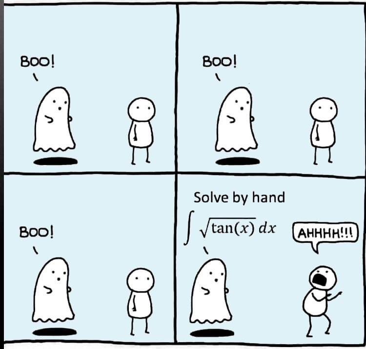
Me at the beginning of every meeting

A bit late. Compliments to Chris for sharing.

can you relate?

Can you solve it?
Several of the colormaps are great for a 256 color surface plot, but aren't well optimized for extracting m colors for plotting several independent lines. The issue is that many colormaps have start/end colors that are too similar or are suboptimal colors for lines. There are certainly many workarounds for this, but it would be a great quality of life to adjust that directly when calling this.
Example:
x = linspace(0,2*pi,101)';
y = [1:6].*cos(x);
figure; plot(x,y,'LineWidth',2); grid on; axis tight;
And now if I wanted to color these lines, I could use something like turbo(6) or gray(6) and then apply it using colororder.
colororder(turbo(6))
But my issue is that the ends of the colormap are too similar. For other colormaps, you may get lines that are too light to be visible against the white background. There are plenty of workarounds, with my preference being to create extra colors and truncate that before using colororder.
cmap = turbo(8); cmap = cmap(2:end-1,:); % Truncate the end colors
figure; plot(x,y,'LineWidth',2); grid on; axis tight;
colororder(cmap)
I think it would be really awesome to add some name-argument input pair to these colormaps that can specify the range you want so this could even be done inside the colororder calling if desired. An example of my proposed solution would look something like this:
cmap = turbo(6,'Range',[0.1 0.8]); % Proposed idea to add functionality
Where in this scenario, the resulting colormap would be 6 equally spaced colors that range from 10% to 80% of the total color range. This would be especially nice because you could more quickly modify the range of colors, or you could set the limits regardless of whether you need to plot 3, 6, or 20 lines.

2 x 2 행렬의 행렬식은
- 행렬의 두 row 벡터로 정의되는 평행사변형의 면적입니다.
- 물론 두 column 벡터로 정의되는 평행사변형의 면적이기도 합니다.
- 좀 더 정확히는 signed area입니다. 면적이 음수가 될 수도 있다는 뜻이죠.
- 행렬의 두 행(또는 두 열)을 맞바꾸면 행렬식의 부호도 바뀌고 면적의 부호도 바뀌어야합니다.
일반적으로 n x n 행렬의 행렬식은
- 각 row 벡터(또는 각 column 벡터)로 정의되는 N차원 공간의 평행면체(?)의 signed area입니다.
- 제대로 이해하려면 대수학의 개념을 많이 가지고 와야 하는데 자세한 설명은 생략합니다.(=저도 모른다는 뜻)
- 더 자세히 알고 싶으시면 수학하는 만화의 '넓이 이야기' 편을 추천합니다.
- 수학적인 정의를 알고 싶으시면 위키피디아를 보시면 됩니다.

- 이렇게 생겼습니다. 좀 무섭습니다.
아래 코드는...
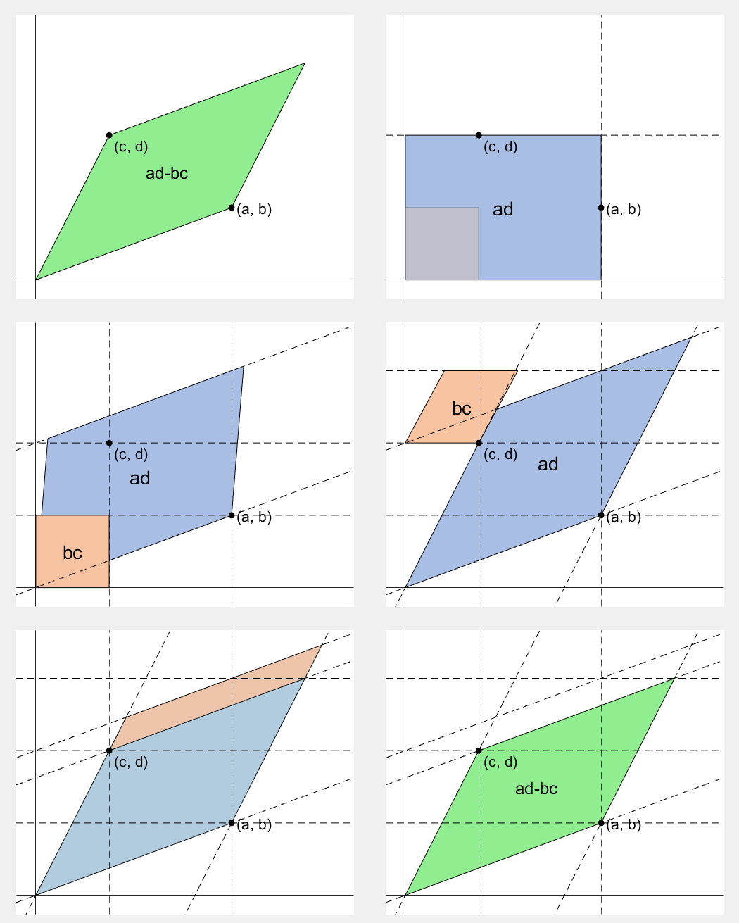
- 2 x 2 행렬에 대해서 이것을 수식 없이 그림만으로 증명하는 과정입니다.
- gif 생성에는 ScreenToGif를 사용했습니다. (gif 만들기엔 이게 킹왕짱인듯)
Determinant of 2 x 2 matrix is...
- An area of a parallelogram defined by two row vectors.
- Of course, same one defined by two column vectors.
- Precisely, a signed area, which means area can be negative.
- If two rows (or columns) are swapped, both the sign of determinant and area change.
More generally, determinant of n x n matrix is...
- Signed area of parallelepiped defined by rows (or columns) of the matrix in n-dim space.
- For a full understanding, a lot of concepts from abstract algebra should be brought, which I will not write here. (Cuz I don't know them.)
- For a mathematical definition of determinant, visit wikipedia.

- A little scary, isn't it?
The code below is...
- A process to prove the equality of the determinant of 2 x 2 matrix and the area of parallelogram.
- ScreenToGif is used to generate gif animation (which is, to me, the easiest way to make gif).
% 두 점 (a, b), (c, d)의 좌표
a = 4;
b = 1;
c = 1;
d = 3;
% patch 색 pre-define
lightgreen = [144, 238, 144]/255;
lightblue = [169, 190, 228]/255;
lightorange = [247, 195, 160]/255;
% animation params.
anim_Nsteps = 30;
% create window
figure('WindowStyle','docked')
ax = axes;
ax.XAxisLocation = 'origin';
ax.YAxisLocation = 'origin';
ax.XTick = [];
ax.YTick = [];
hold on
ax.XLim = [-.4, a+c+1];
ax.YLim = [-.4, b+d+1];
% create ad-bc patch
area = patch([0, a, a+c, c], [0, b, b+d, d], lightgreen);
p_ab = plot(a, b, 'ko', 'MarkerFaceColor', 'k');
p_cd = plot(c, d, 'ko', 'MarkerFaceColor', 'k');
p_ab.UserData = text(a+0.1, b, '(a, b)', 'FontSize',16);
p_cd.UserData = text(c+0.1, d-0.2, '(c, d)', 'FontSize',16);
area.UserData = text((a+c)/2-0.5, (b+d)/2, 'ad-bc', 'FontSize', 18);
pause
%% Is this really ad-bc?
area.UserData.String = 'ad-bc...?';
pause
%% fade out ad-bc
fadeinout(area, 0)
area.UserData.Visible = 'off';
pause
%% fade in ad block
rect_ad = patch([0, a, a, 0], [0, 0, d, d], lightblue, 'EdgeAlpha', 0, 'FaceAlpha', 0);
uistack(rect_ad, 'bottom');
fadeinout(rect_ad, 1, t_pause=0.003)
draw_gridline(rect_ad, ["23", "34"])
rect_ad.UserData = text(mean(rect_ad.XData), mean(rect_ad.YData), 'ad', 'FontSize', 20, 'HorizontalAlignment', 'center');
pause
%% fade-in bc block
rect_bc = patch([0, c, c, 0], [0, 0, b, b], lightorange, 'EdgeAlpha', 0, 'FaceAlpha', 0);
fadeinout(rect_bc, 1, t_pause=0.0035)
draw_gridline(rect_bc, ["23", "34"])
rect_bc.UserData = text(b/2, c/2, 'bc', 'FontSize', 20, 'HorizontalAlignment', 'center');
pause
%% slide ad block
patch_slide(rect_ad, ...
[0, 0, 0, 0], [0, b, b, 0], t_pause=0.004)
draw_gridline(rect_ad, ["12", "34"])
pause
%% slide ad block
patch_slide(rect_ad, ...
[0, 0, d/(d/c-b/a), d/(d/c-b/a)],...
[0, 0, b/a*d/(d/c-b/a), b/a*d/(d/c-b/a)], t_pause=0.004)
draw_gridline(rect_ad, ["14", "23"])
pause
%% slide bc block
uistack(p_cd, 'top')
patch_slide(rect_bc, ...
[0, 0, 0, 0], [d, d, d, d], t_pause=0.004)
draw_gridline(rect_bc, "34")
pause
%% slide bc block
patch_slide(rect_bc, ...
[0, 0, a, a], [0, 0, 0, 0], t_pause=0.004)
draw_gridline(rect_bc, "23")
pause
%% slide bc block
patch_slide(rect_bc, ...
[d/(d/c-b/a), 0, 0, d/(d/c-b/a)], ...
[b/a*d/(d/c-b/a), 0, 0, b/a*d/(d/c-b/a)], t_pause=0.004)
pause
%% finalize: fade out ad, bc, and fade in ad-bc
rect_ad.UserData.Visible = 'off';
rect_bc.UserData.Visible = 'off';
fadeinout([rect_ad, rect_bc, area], [0, 0, 1])
area.UserData.String = 'ad-bc';
area.UserData.Visible = 'on';
%% functions
function fadeinout(objs, inout, options)
arguments
objs
inout % 1이면 fade-in, 0이면 fade-out
options.anim_Nsteps = 30
options.t_pause = 0.003
end
for alpha = linspace(0, 1, options.anim_Nsteps)
for i = 1:length(objs)
switch objs(i).Type
case 'patch'
objs(i).FaceAlpha = (inout(i)==1)*alpha + (inout(i)==0)*(1-alpha);
objs(i).EdgeAlpha = (inout(i)==1)*alpha + (inout(i)==0)*(1-alpha);
case 'constantline'
objs(i).Alpha = (inout(i)==1)*alpha + (inout(i)==0)*(1-alpha);
end
pause(options.t_pause)
end
end
end
function patch_slide(obj, x_dist, y_dist, options)
arguments
obj
x_dist
y_dist
options.anim_Nsteps = 30
options.t_pause = 0.003
end
dx = x_dist/options.anim_Nsteps;
dy = y_dist/options.anim_Nsteps;
for i=1:options.anim_Nsteps
obj.XData = obj.XData + dx(:);
obj.YData = obj.YData + dy(:);
obj.UserData.Position(1) = mean(obj.XData);
obj.UserData.Position(2) = mean(obj.YData);
pause(options.t_pause)
end
end
function draw_gridline(patch, where)
ax = patch.Parent;
for i=1:length(where)
v1 = str2double(where{i}(1));
v2 = str2double(where{i}(2));
x1 = patch.XData(v1);
x2 = patch.XData(v2);
y1 = patch.YData(v1);
y2 = patch.YData(v2);
if x1==x2
xline(x1, 'k--')
else
fplot(@(x) (y2-y1)/(x2-x1)*(x-x1)+y1, [ax.XLim(1), ax.XLim(2)], 'k--')
end
end
end
Happy year of the dragon.

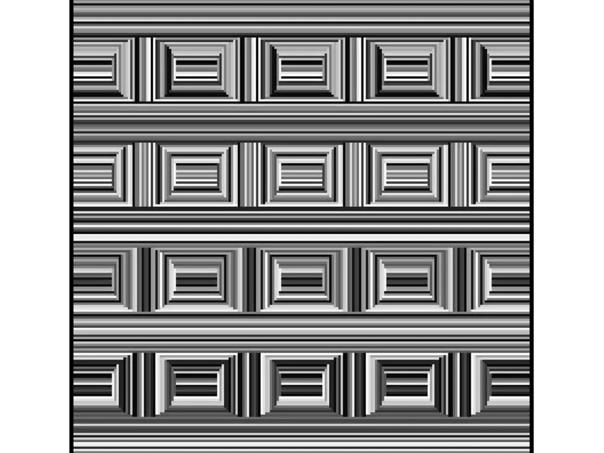
Can you see them?
I have been procrastinating on schoolwork by looking at all the amazing designs created in the last MATLAB Flipbook Mini Hack! They are just amazing. The voting is over but what are y'all's personal favorites? Mine is the flapping butterfly, it is for sure a creation I plan to share with others in the future!

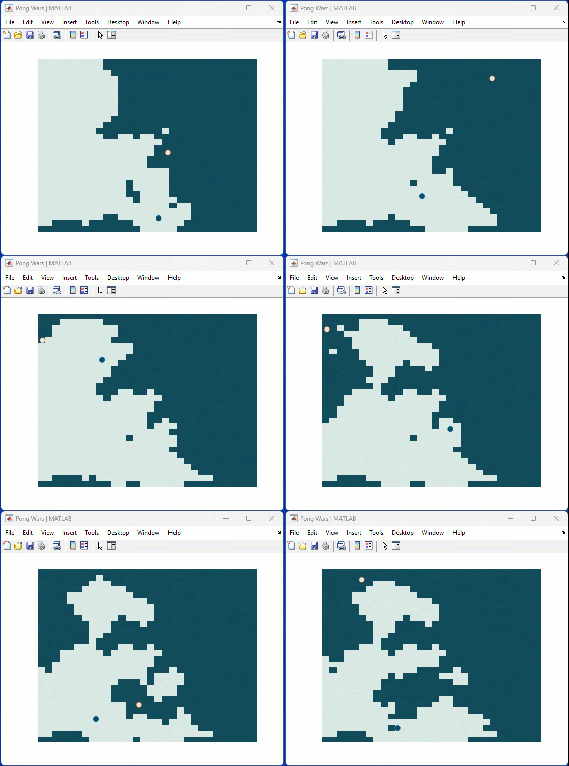
One of my colleauges, Michio, recently posted an implementation of Pong Wars in MATLAB
- Here's the code on GitHub.https://lnkd.in/gZG-AsFX
- If you want to open with MATLAB Online, click here https://lnkd.in/gahrTMW5
- He saw this first here: https://lnkd.in/gu_Z-Pks
Making me wonder about variations. What might the resulting patterns look with differing numbers of balls? Different physics etc?

I recently wrote about the new ODE solution framework in MATLAB over the The MATLAB Blog The new solution framework for Ordinary Differential Equations (ODEs) in MATLAB R2023b » The MATLAB Blog - MATLAB & Simulink (mathworks.com)
This was a very popular post at the time - many thousands of views. Clearly everyone cares about ODEs in MATLAB.
This made me wonder. If you could wave a magic wand, what ODE functionality would you have next and why?
Is there a reason for TMW not to invest in 3D polyshapes? Is the mathematical complexity of having all the same operations in 3D (union, intersection, subtract,...) prohibitive?
Quick answer: Add set(hS,'Color',[0 0.4470 0.7410]) to code line 329 (R2023b).
Explanation: Function corrplot uses functions plotmatrix and lsline. In lsline get(hh(k),'Color') is called in for cycle for each line and scatter object in axes. Inside the corrplot it is also called for all axes, which is slow. However, when you first set the color to any given value, internal optimization makes it much faster. I chose [0 0.4470 0.7410], because it is a default color for plotmatrix and corrplot and this setting doesn't change a behavior of corrplot.
Suggestion for a better solution: Add the line of code set(hS,'Color',[0 0.4470 0.7410]) to the function plotmatrix. This will make not only corrplot faster, but also any other possible combinations of plotmatrix and get functions called like this:
h = plotmatrix(A);
% set(h,'Color',[0 0.4470 0.7410])
for k = 1:length(h(:))
get(h(k),'Color');
end
I think it would be a really great feature to be able to add an Alpha property to the basic "Line" class in MATLAB plots. I know that I have previously had to resort to using Patch to be able to plot semitransparent lines, but there are also so many other functions that rely on the "Line" class.
For example, if you want to make a scatter plot from a table with things specified into groups, you can use ScatterHistogram or gscatter but since gscatter uses the Line class, you can't adjust the marker transparency. So if you don't want the histograms, you are stuck with manually separating it and using scatter with hold on.
Hi Guys
Posting this based on a thought I had, so I don't really ahve any code however I would like to know if the thought process is correct and/or relatively accurate.
Consider a simple spring mass system which only allows compression on the spring however when there is tension the mass should move without the effect of the spring distrupting it, thus the mass is just thrown vertically upwards.
The idea which I came up with for such a system is to have two sets of dfferential equations, one which represents the spring system and another which presents a mass in motion without the effects of the spring.
Please refer to the below basic outline of the code which I am proposing. I believe that this may produce relatively decent results. The code essentially checks if there is tension in the system if there is it then takes the last values from the spring mass differential equation and uses it as initial conditions for the differential equation with the mass moving wothout the effects of the spring, this process works in reverse also. The error which would exist is that the initial conditions applied to the system would include effects of the spring. Would there be a better way to code such behaviour?
function xp = statespace(t,x,f,c,k,m)
if (k*x(1)) positive #implying tension
**Use last time step as initial conditions**
**differential equation of a mass moving""
end
if x(1) negative #implying that the mass in now moving down therefore compression in spring
**Use last time step as initial conditions**
**differential equation for a spring mass system**
end
end
Seeing a colleague make this mistake (one I've had to fix multiple times in other's work too) makes me want to ask the community: would you like the awgn() function/blocks to give the option for creating a SNR at the bandwidth of the signal? Your typical flow is something like this:
- Create a signal, usually at some nominal upsampling factor (e.g., 4) such that it's now nicely over sampled, especially if you're using a RRC or similar pulse shaping filter.
- Potentially add a frequency offset (which might make the sample frequency even higher)
- Add AWGN channel model for a desired SNR
- Put this into your detector/receiver model
The problem is, when someone says, "I'm detecting XYZ at foo SNR," it should not magically improve as a function of the oversample. The problem isn't that awgn() generates white noise, that's what it's supposed to do and the typical receiver has noise across the entire band. The problem is that SNR is most properly defined as the signal power over the noise power spectral density times the signal's noise equivalent bandwidth. Now I looked and there's no handy function for computing NEBW for an input signal (there's just a function for assessing analysis windows). In practice it can get a bit tricky. The occupied bandwidth or HPBW are often close enough to the NEBW, we're usually not haggling over hundredths of a dB. So, in my not so humble opinion, the "measured" flag for awgn() should give an option for bandwidth matching or at least document the behavior better in the help page. All too often I'm seeing 3-6 (or worse) dB errors because people aren't taking the signal's bandwidth into account.

Share your fun photos in the comments!
I know the latest version of MATLAB R2023b has this feature already, put it should be added to R2023a as well because of its simplicity and convenience.
Basically, I want to make a bar graph that lets me name each column in a basic bar graph:
y=[100 99 100 200 200 300 500 800 1000];
x=["0-4" "5-17" "18-29" "30-39" "40-49" "50-64" "65-74" "75-84" "85+"];
bar(x,y)
However, in R2023a, this isn't a feature. I think it should be added because it helps to present data and ideas more clearly and professionally, which is the purpose of a graph to begin with.


