Risultati per
Following on from my previous post The Non-Chaotic Duffing Equation, now we will study the chaotic behaviour of the Duffing Equation
P.s:Any comments/advice on improving the code is welcome.
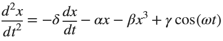
The Original Duffing Equation is the following:
Let 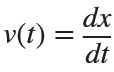 . This implies that
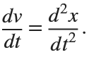
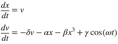
Then we rewrite it as a System of First-Order Equations
Using the substitution  for
for  , the second-order equation can be transformed into the following system of first-order equations:
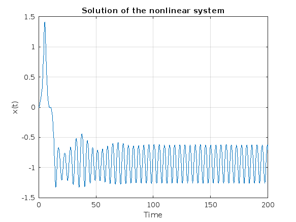
Exploring the Effect of γ.
% Define parameters
gamma = 0.1;
alpha = -1;
beta = 1;
delta = 0.1;
omega = 1.4;
% Define the system of equations
odeSystem = @(t, y) [y(2);
-delta*y(2) - alpha*y(1) - beta*y(1)^3 + gamma*cos(omega*t)];
% Initial conditions
y0 = [0; 0]; % x(0) = 0, v(0) = 0
% Time span
tspan = [0 200];
% Solve the system
[t, y] = ode45(odeSystem, tspan, y0);
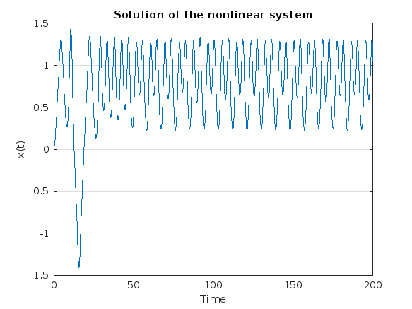
% Plot the results
figure;
plot(t, y(:, 1));
xlabel('Time');
ylabel('x(t)');
title('Solution of the nonlinear system');
grid on;
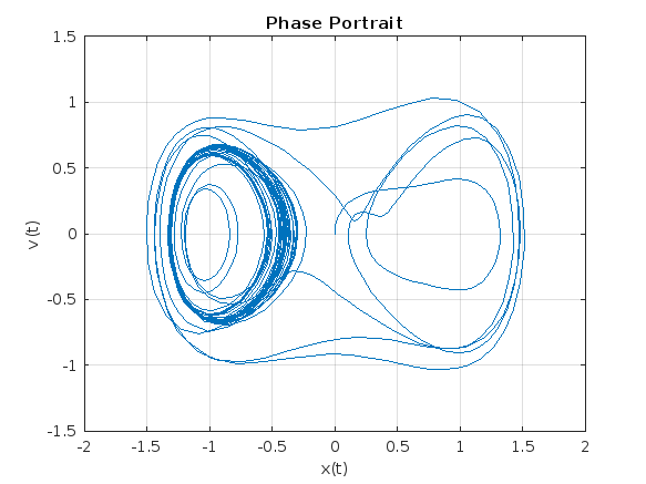
% Plot the phase portrait
figure;
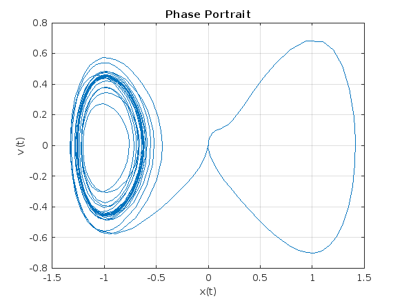
plot(y(:, 1), y(:, 2));
xlabel('x(t)');
ylabel('v(t)');
title('Phase Portrait');
grid on;
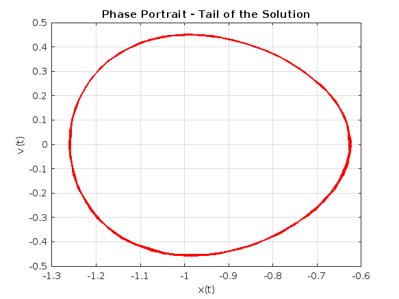
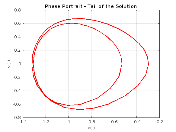
% Define the tail (e.g., last 10% of the time interval)
tail_start = floor(0.9 * length(t)); % Starting index for the tail
tail_end = length(t); % Ending index for the tail
% Plot the tail of the solution
figure;
plot(y(tail_start:tail_end, 1), y(tail_start:tail_end, 2), 'r', 'LineWidth', 1.5);
xlabel('x(t)');
ylabel('v(t)');
title('Phase Portrait - Tail of the Solution');
grid on;
% Define parameters
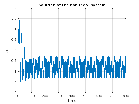
gamma = 0.318;
alpha = -1;
beta = 1;
delta = 0.1;
omega = 1.4;
% Define the system of equations
odeSystem = @(t, y) [y(2);
-delta*y(2) - alpha*y(1) - beta*y(1)^3 + gamma*cos(omega*t)];
% Initial conditions
y0 = [0; 0]; % x(0) = 0, v(0) = 0
% Time span
tspan = [0 800];
% Solve the system
[t, y] = ode45(odeSystem, tspan, y0);
% Plot the results
figure;
plot(t, y(:, 1));
xlabel('Time');
ylabel('x(t)');
title('Solution of the nonlinear system');
grid on;
% Plot the phase portrait
figure;
plot(y(:, 1), y(:, 2));
xlabel('x(t)');
ylabel('v(t)');
title('Phase Portrait');
grid on;
% Define the tail (e.g., last 10% of the time interval)
tail_start = floor(0.9 * length(t)); % Starting index for the tail
tail_end = length(t); % Ending index for the tail
% Plot the tail of the solution
figure;
plot(y(tail_start:tail_end, 1), y(tail_start:tail_end, 2), 'r', 'LineWidth', 1.5);
xlabel('x(t)');
ylabel('v(t)');
title('Phase Portrait - Tail of the Solution');
grid on;
% Define parameters
gamma = 0.338;
alpha = -1;
beta = 1;
delta = 0.1;
omega = 1.4;
% Define the system of equations
odeSystem = @(t, y) [y(2);
-delta*y(2) - alpha*y(1) - beta*y(1)^3 + gamma*cos(omega*t)];
% Initial conditions
y0 = [0; 0]; % x(0) = 0, v(0) = 0
% Time span with more points for better resolution
tspan = linspace(0, 200,2000); % Increase the number of points
% Solve the system
[t, y] = ode45(odeSystem, tspan, y0);
% Plot the results
figure;
plot(t, y(:, 1));
xlabel('Time');
ylabel('x(t)');
title('Solution of the nonlinear system');
grid on;
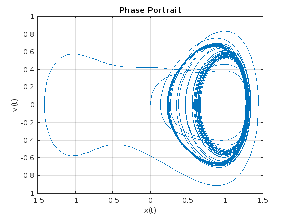
% Plot the phase portrait
figure;
plot(y(:, 1), y(:, 2));
xlabel('x(t)');
ylabel('v(t)');
title('Phase Portrait');
grid on;
% Define the tail (e.g., last 10% of the time interval)
tail_start = floor(0.9 * length(t)); % Starting index for the tail
tail_end = length(t); % Ending index for the tail
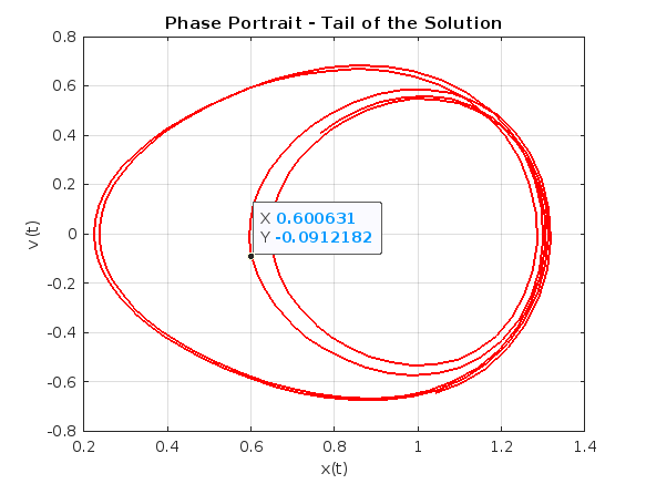
% Plot the tail of the solution
figure;
plot(y(tail_start:tail_end, 1), y(tail_start:tail_end, 2), 'r', 'LineWidth', 1.5);
xlabel('x(t)');
ylabel('v(t)');
title('Phase Portrait - Tail of the Solution');
grid on;
ax = gca;
chart = ax.Children(1);
datatip(chart,0.5581,-0.1126);
% Define parameters
gamma = 0.35;
alpha = -1;
beta = 1;
delta = 0.1;
omega = 1.4;
% Define the system of equations
odeSystem = @(t, y) [y(2);
-delta*y(2) - alpha*y(1) - beta*y(1)^3 + gamma*cos(omega*t)];
% Initial conditions
y0 = [0; 0]; % x(0) = 0, v(0) = 0
% Time span with more points for better resolution
tspan = linspace(0, 400,3000); % Increase the number of points
% Solve the system
[t, y] = ode45(odeSystem, tspan, y0);
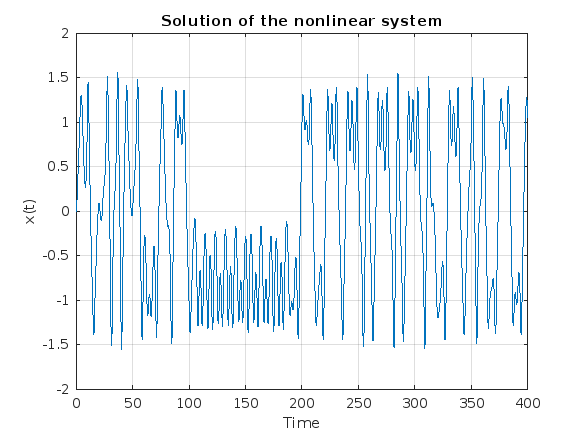
% Plot the results
figure;
plot(t, y(:, 1));
xlabel('Time');
ylabel('x(t)');
title('Solution of the nonlinear system');
grid on;
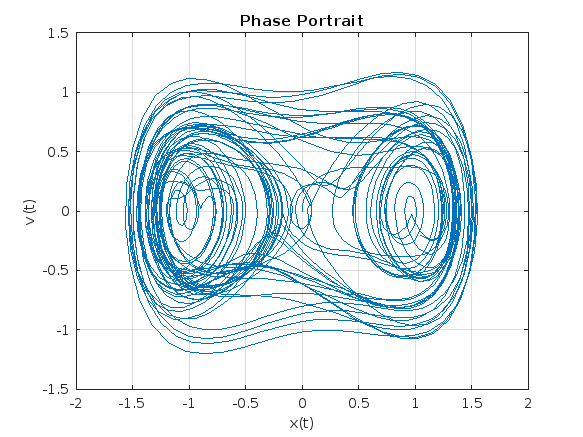
% Plot the phase portrait
figure;
plot(y(:, 1), y(:, 2));
xlabel('x(t)');
ylabel('v(t)');
title('Phase Portrait');
grid on;
% Define the tail (e.g., last 10% of the time interval)
tail_start = floor(0.9 * length(t)); % Starting index for the tail
tail_end = length(t); % Ending index for the tail
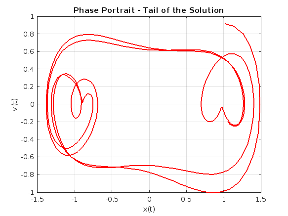
% Plot the tail of the solution
figure;
plot(y(tail_start:tail_end, 1), y(tail_start:tail_end, 2), 'r', 'LineWidth', 1.5);
xlabel('x(t)');
ylabel('v(t)');
title('Phase Portrait - Tail of the Solution');
grid on;
An attractor is called strange if it has a fractal structure, that is if it has non-integer Hausdorff dimension. This is often the case when the dynamics on it are chaotic, but strange nonchaotic attractors also exist. If a strange attractor is chaotic, exhibiting sensitive dependence on initial conditions, then any two arbitrarily close alternative initial points on the attractor, after any of various numbers of iterations, will lead to points that are arbitrarily far apart (subject to the confines of the attractor), and after any of various other numbers of iterations will lead to points that are arbitrarily close together. Thus a dynamic system with a chaotic attractor is locally unstable yet globally stable: once some sequences have entered the attractor, nearby points diverge from one another but never depart from the attractor.
The term strange attractor was coined by David Ruelle and Floris Takens to describe the attractor resulting from a series of bifurcations of a system describing fluid flow. Strange attractors are often differentiable in a few directions, but some are like a Cantor dust, and therefore not differentiable. Strange attractors may also be found in the presence of noise, where they may be shown to support invariant random probability measures of Sinai–Ruelle–Bowen type.
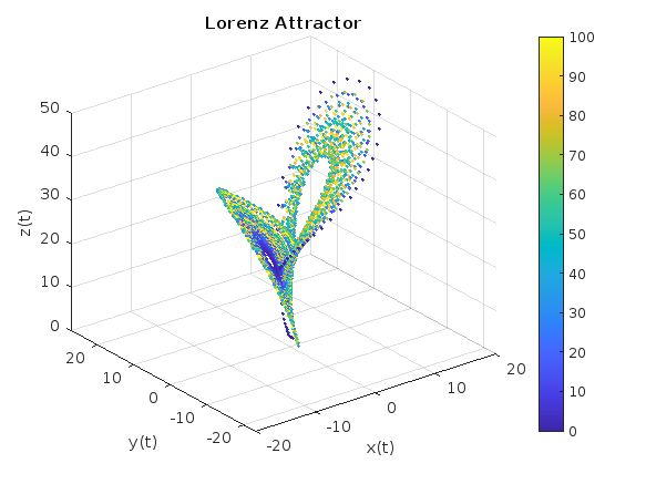
Lorenz
% Lorenz Attractor Parameters
sigma = 10;
beta = 8/3;
rho = 28;
% Lorenz system of differential equations
f = @(t, a) [-sigma*a(1) + sigma*a(2);
rho*a(1) - a(2) - a(1)*a(3);
-beta*a(3) + a(1)*a(2)];
% Time span
tspan = [0 100];
% Initial conditions
a0 = [1 1 1];
% Solve the system using ode45
[t, a] = ode45(f, tspan, a0);
% Plot using scatter3 with time-based color mapping
figure;
scatter3(a(:,1), a(:,2), a(:,3), 5, t, 'filled'); % 5 is the marker size
title('Lorenz Attractor');
xlabel('x(t)');
ylabel('y(t)');
zlabel('z(t)');
grid on;
colorbar; % Add a colorbar to indicate the time mapping
view(3); % Set the view to 3D
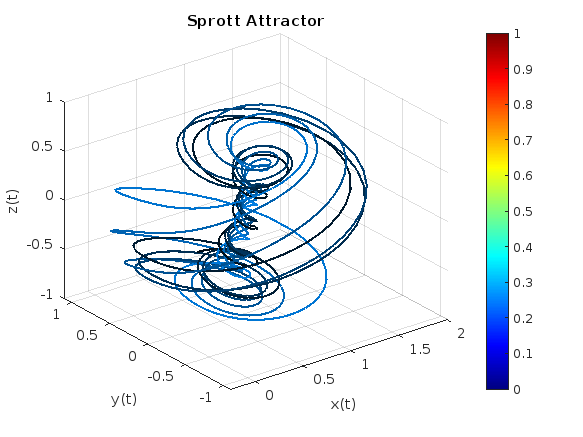
Sprott
% Define the parameters
a = 2.07;
b = 1.79;
% Define the system of differential equations
dynamics = @(t, X) [ ...
X(2) + a * X(1) * X(2) + X(1) * X(3); % dx/dt
1 - b * X(1)^2 + X(2) * X(3); % dy/dt
X(1) - X(1)^2 - X(2)^2 % dz/dt
];
% Initial conditions
X0 = [0.63; 0.47; -0.54];
% Time span
tspan = [0 100];
% Solve the system using ode45
[t, X] = ode45(dynamics, tspan, X0);
% Plot the results with color gradient
figure;
colormap(jet); % Set the colormap
c = linspace(1, 10, length(t)); % Color data based on time
% Create a 3D line plot with color based on time
for i = 1:length(t)-1
plot3(X(i:i+1,1), X(i:i+1,2), X(i:i+1,3), 'Color', [0 0.5 0.9]*c(i)/10, 'LineWidth', 1.5);
hold on;
end
% Set plot properties
title('Sprott Attractor');
xlabel('x(t)');
ylabel('y(t)');
zlabel('z(t)');
grid on;
colorbar; % Add a colorbar to indicate the time mapping
view(3); % Set the view to 3D
hold off;
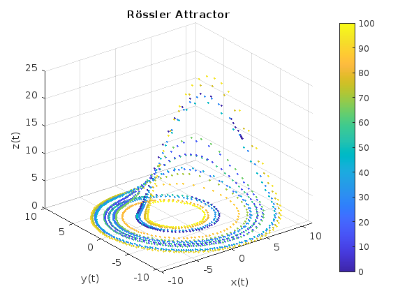
Rössler
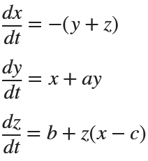
% Define the parameters
a = 0.2;
b = 0.2;
c = 5.7;
% Define the system of differential equations
dynamics = @(t, X) [ ...
-(X(2) + X(3)); % dx/dt
X(1) + a * X(2); % dy/dt
b + X(3) * (X(1) - c) % dz/dt
];
% Initial conditions
X0 = [10.0; 0.00; 10.0];
% Time span
tspan = [0 100];
% Solve the system using ode45
[t, X] = ode45(dynamics, tspan, X0);
% Plot the results
figure;
scatter3(X(:,1), X(:,2), X(:,3), 5, t, 'filled');
title('Rössler Attractor');
xlabel('x(t)');
ylabel('y(t)');
zlabel('z(t)');
grid on;
colorbar; % Add a colorbar to indicate the time mapping
view(3); % Set the view to 3D
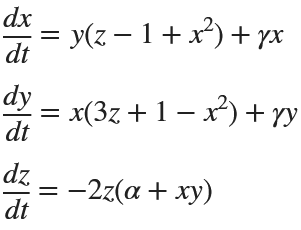
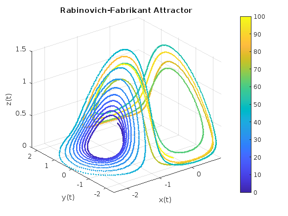
Rabinovich-Fabrikant
%% Parameters for Rabinovich-Fabrikant Attractor
alpha = 0.14;
gamma = 0.10;
dt = 0.01;
num_steps = 5000;
% Initial conditions
x0 = -1;
y0 = 0;
z0 = 0.5;
% Preallocate arrays for performance
x = zeros(1, num_steps);
y = zeros(1, num_steps);
z = zeros(1, num_steps);
% Set initial values
x(1) = x0;
y(1) = y0;
z(1) = z0;
% Generate the attractor
for i = 1:num_steps-1
x(i+1) = x(i) + dt * (y(i)*(z(i) - 1 + x(i)^2) + gamma*x(i));
y(i+1) = y(i) + dt * (x(i)*(3*z(i) + 1 - x(i)^2) + gamma*y(i));
z(i+1) = z(i) + dt * (-2*z(i)*(alpha + x(i)*y(i)));
end
% Create a time vector for color mapping
t = linspace(0, 100, num_steps);
% Plot using scatter3
figure;
scatter3(x, y, z, 5, t, 'filled'); % 5 is the marker size
title('Rabinovich-Fabrikant Attractor');
xlabel('x(t)');
ylabel('y(t)');
zlabel('z(t)');
grid on;
colorbar; % Add a colorbar to indicate the time mapping
view(3); % Set the view to 3D
References