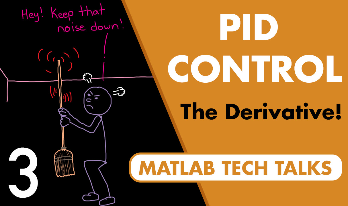
Expanding Beyond a Simple Derivative | Understanding PID Control, Part 3
From the series: Understanding PID Control
Brian Douglas
This video describes how to make an ideal PID controller more robust when controlling real systems that don’t behave like ideal linear models. Noise is generated by sensors and is present in every system. The derivative in an ideal PID controller amplifies high-frequency noise. Even if that noise is relatively low amplitude, the derivative will sense it and possibly amplify it enough to impact the controller. To protect against high-frequency noise impacting the system, you can modify the derivative path with a low pass filter to reduce the noise before it causes any problems.
Published: 9 Jul 2018
Let's continue to expand our ideal PID controller and see if we can make it even more robust when trying to control real systems that don't behave like ideal linear models. In the last video, we looked at how an actuator can saturate. And we tacked on some anti-windup logic to deal with that. In this video, we're going to focus our attention on the derivative and look at how the device that is sensing the true state of the system and producing a measured state that the controller can use can add noise into our feedback loop. I'm Brian, and welcome to a MATLAB Tech Talk.
Noise is a random disturbance on a signal. And when you're dealing with sensors, both mechanical and electronic sensors, it is unavoidable. The generic term "noise" refers to the summation of different noises created from different sources that stem from things like the environment it's operating in, which is both naturally occurring noise and man-made noise, the specific implementation of the electronics, and from manufacturing defects. They can exist at very specific frequencies or be spread out across the spectrum.
For example, if the noise has equal intensities at different frequencies, then it's called white noise, which you have probably seen and heard as static in a nonexistent radio or TV station. But beyond white noise, there are tons of things that can cause noise in your system. And they have cool names like thermal noise, shot noise, flicker noise, burst noise, and coupled noise, to just name a few. And the descriptions of each of these are beyond the scope of this video.
But the thing to take away from this is that they all produce these tiny shifts in voltage over a wide range of frequencies, which in turn produces shifts in the measurement itself. Now, it's easy to see how large amplitude or really loud noise could impact a system. But what isn't as obvious is how small-amplitude, quiet noise, but really high frequency, can also cause problems.
What the sensor is measuring might be a nice, smooth quantity, like a slowly rising temperature. But due to sensor noise, the measurement might be jagged, with tiny fluctuations that deviate from the true temperature, even if they're so small you can't initially tell just by looking at the data with your own eye.
An easy way to demonstrate this is to take a picture with your cell phone. But instead of a busy image, where you might not notice some really subtle noise, take a black image by laying it down on a flat surface so that no light can get in. I took a dark image with my cell phone, and to show you what this noise looks like, I'll use MATLAB to view the image.
At first glance, the image looks like a perfectly black picture but there are slight variations in those dark pixels. We can confirm that by making the image brighter by multiplying each pixel value by 50. And you can see that it's obvious that there's some low-amplitude random noise throughout this image.
Now, this little bit of noise doesn't impact the look of the image much, especially if it's a bright, vibrant image. So it stands to reason that low-amplitude noise won't impact our control system much either. It'll be down in the noise, as they say.
And that's true for some control laws. As long as the noise is low amplitude, then it won't impact the system much. But that's not true for our ideal PID controller, because this has a pure derivative. Derivatives amplify high-frequency signals and can take those tiny, barely noticeable wiggles and amplify them to values that can impact our system.
Let's see if we can figure out why that is. Let's look at a low-frequency noise signal, just a pure sine wave. The slope of the signal is the derivative. And if we look at the point where the signal has the steepest slope and draw a yellow line, we can get a visual indication of what value the derivative will return. The steeper the line, the higher the derivative.
Now let's look at how the slope changes for a high-frequency signal. The amplitude of the noise hasn't changed. But the increase in frequency generated a steeper slope. We can reduce the amplitude of the noise signal and get back to a slope or a derivative that is similar to the low-frequency signal. And this is the general idea we'll use later-- lower the amplitude of high-frequency noise so that the derivative isn't too large.
And if we increase the frequency even more, the slope gets steeper. And we'll have to lower the amplitude to account for that. So you can see that if you leave really, really high-frequency noise in your system, the derivative path will see that noise even if it's really small, and amplify it, and cause you issues.
We can look at the derivative and see that the amplification of high frequencies also makes sense mathematically. Any signal can be defined as a summation of an infinite number of sine waves. And this is what you're doing when you take a Fourier transform of a signal.
For the purpose of this example, we only need to look at a single frequency, where A is the amplitude, omega A is the frequency in radians per second, and "phee," or "phi," is the phase. And if we take the derivative of this sine wave, we get a new sine wave at the exact same frequency, but shifted in phase by 90 degrees and with a new amplitude, A times omega A.
And from here, it's easy to see that if omega A is greater than 1 radian per second, the amplitude got larger. And if omega A is less than 1 radian per second, the amplitude got smaller. And if we plot this magnitude change, it will look like this sloped yellow line, where higher frequencies create higher-amplitude signals, and lower frequencies create lower-amplitude signals.
So we want a filter that can block frequencies above a certain point from entering our derivative and causing problems. This point is called the cutoff frequency. And as designers, we have the choice of where to place it. For example, do we place it at a high frequency and block just the orange section or place it lower and block the green section?
All right, let's add our filter to the derivative path and start to talk about what this looks like. Ideally, you want a filter that can remove all of the noise and perfectly pass through all of the signal. But this isn't something that can be achieved in practice.
Luckily, for a lot of applications, to noise across the spectrum is relatively low amplitude or low power. And the signal you're interested in keeping has comparatively large power and low frequency. In this case, the low-frequency noise doesn't really impact the derivative much if the amplitude is small. And therefore, we can often remove all of the bothersome noise to our derivative simply by blocking or attenuating just the high-frequency information.
And the simplest way to do that is with a first-order low-pass filter. This is a filter, as the name suggests, that will allow frequencies below the cutoff point to pass through mostly unchanged and will attenuate or lower the amplitude of frequencies above the cutoff point. It doesn't remove the noise entirely. It just makes it smaller so that even after we amplify it through the derivative, it won't impact our system much.
And the key aspect of this filter is determining where to put the cutoff frequency so that you remove as much high-frequency noise as possible without impinging on the frequencies that are actually in the signal you care about. We'll talk more about that when we talk tuning in a future video.
Now, before I close out this video, I want to briefly show you the structure of this low-pass filter and derivative combination, mostly so that I can show you a really cool way to implement the derivative portion of the PID controller using not a derivative, but using an integral instead. This section requires some knowledge of Laplace domain transfer functions. But if you're not familiar with them, that's OK. I think you'll still get something out of hearing the concepts. I'll provide a simple cheat sheet to help interpret the various transfer functions that we're going to be looking at, though.
S is the Laplace domain representation of a derivative. And the inverse, 1 over S, is the representation of an integral. And N divided by S plus N is a low-pass filter, first order, where the number N is the cutoff frequency in radians per second.
So if you see the transfer function 10 over S plus 10, this is a low-pass filter with cutoff frequency at 10 radians per second. Also, N over S plus N isn't the only popular form of the first-order low-pass filter. We can divide the top and bottom by N to get 1 divided by 1 over N times S plus 1.
And since the inverse of frequency is time, this form of the equation allows you to specify the time constant of the filter rather than the cutoff frequency. Here, I'm using tau to represent the time constant. But you may also see T or TF, depending on the industry that you're in.
All right, so using these definitions, we have a low-pass filter and a derivative. And the transfer function of these combined systems is the product of the two, or S times N over S plus N. And from here, we could choose a cutoff frequency and implement a digital version of this in our PID code.
But I want to show you an alternative approach to implementing this logic. Instead of a low-pass filter in series with a derivative, we can create a feedback loop with N in the forward path and an integral in the feedback path. This might not look like the same logic. But we can reduce this block diagram to a single transfer function, N over 1 plus N times 1 over S, and then move the S around to get S times N over S plus N, which is exactly equal to what we had before.
If you're not familiar with block diagram reduction or how we went from the feedback system to a transfer function, N over 1 plus N times 1 over S, I'll quickly go through an algebraic derivation that you can walk through on your own if you pause this video.
So this is an interesting result. You have the choice to implement a low-pass filter and a derivative or a feedback loop with an integral in the feedback path. They are going to produce the exact same effect. So why implement one versus the other?
Well, I think it comes down to this. Writing out the filter and derivative explicitly makes your code easy to read and understand. So I think it's preferred. However, it takes more math operations and more computer memory to accomplish this. The integral in the feedback path is a more efficient computation. So which way you implement it depends on what you're going for, easy-to-read code or efficient algorithms.
So at this point, let's go over to MATLAB and launch Simulink. We just need a blank model to start. And I'll add the PID controller block to it. When you double-click this block to open up the parameters, you'll notice that you have control over both the derivative gain and the filter coefficient, N.
And if you look at the formula that Simulink is using, it isn't a pure derivative. It's the formula for the filter derivative that we just described. So hopefully this cleared up any confusion you might have about why the derivative path is not just a pure derivative, and it gives you a better insight into what the filter coefficient is and how it protects your system from high-frequency noise.
In the next video, we're going to get into some ways to tune your controller to get the performance that you want. So if you don't want to miss the next Tech Talk, Don't forget to subscribe to this channel. Also, if you want to check out my channel, Control System Lectures, I cover more control theory topics there as well. Thanks for watching, and I'll see you next time.
Related Products
Learn More


Seleziona un sito web
Seleziona un sito web per visualizzare contenuto tradotto dove disponibile e vedere eventi e offerte locali. In base alla tua area geografica, ti consigliamo di selezionare: United States.
Puoi anche selezionare un sito web dal seguente elenco:
Americhe
- América Latina (Español)
- Canada (English)
- United States (English)
Europa
- Belgium (English)
- Denmark (English)
- Deutschland (Deutsch)
- España (Español)
- Finland (English)
- France (Français)
- Ireland (English)
- Italia (Italiano)
- Luxembourg (English)
- Netherlands (English)
- Norway (English)
- Österreich (Deutsch)
- Portugal (English)
- Sweden (English)
- Switzerland
- United Kingdom (English)