pzmap
Mappa a polo zero del sistema dinamico
Sintassi
Descrizione
[ restituisce i poli del sistema e gli zeri di trasmissione del modello di sistema dinamico p,z] = pzmap(sys)sys.
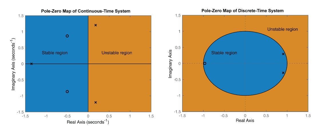
La figura seguente mostra le mappe a polo zero per un modello lineare a tempo variabile a tempo continuo (a sinistra) e a tempo discreto (a destra).
Nei sistemi a tempo continuo, tutti i poli sul piano s complesso devono trovarsi nel semipiano sinistro (regione blu) per garantire la stabilità. Il sistema è marginalmente stabile se i poli distinti si trovano sull'asse immaginario, ossia se le parti reali dei poli sono pari a zero.
Nei sistemi a tempo discreto, tutti i poli nel piano z complesso devono trovarsi all'interno del cerchio unitario (regione blu). Il sistema è marginalmente stabile se uno o più poli si trovano sul cerchio unitario.
pzmap( traccia una mappa a polo zero per sys)sys. Nel grafico, x e o rappresentano rispettivamente i poli e gli zeri. Per i sistemi SISO, pzmap traccia i poli e gli zeri del sistema. Per i sistemi MIMO, pzmap traccia i poli del sistema e gli zeri di trasmissione.
Esempi
Tracciare i poli e gli zeri del sistema a tempo continuo rappresentato dalla seguente funzione di trasferimento:
H = tf([2 5 1],[1 3 5]);
pzmap(H)
grid on
Attivando la griglia vengono visualizzate le linee del rapporto di smorzamento costante (zeta) e le linee a frequenza naturale costante (wn). Questo sistema presenta due zeri reali, contrassegnati da o sul grafico. Il sistema presenta inoltre una coppia di poli complessi, contrassegnati da x.
Tracciare la mappa a polo zero di un modello stato-spazio identificato a tempo discreto (idss). In concreto, è possibile ottenere un modello idss mediante una stima basata sulle misurazioni di input-output di un sistema. Per questo esempio, creare un modello dai dati stato-spazio.
A = [0.1 0; 0.2 -0.9];
B = [.1 ; 0.1];
C = [10 5];
D = [0];
sys = idss(A,B,C,D,'Ts',0.1);
Esaminare la mappa a polo zero.
pzmap(sys)

I poli del sistema sono contrassegnati da x, mentre gli zeri sono contrassegnati da o.
Per questo esempio, caricare un array 3x1 di modelli della funzione di trasferimento.
load("tfArray.mat","sys");
size(sys)
3x1 array of transfer functions.
Each model has 1 outputs and 1 inputs.
Tracciare i poli e gli zeri di ciascun modello nell'array con colori distinti. Per questo esempio, utilizzare il rosso per il primo modello nell'array, il verde per il secondo e il blu per il terzo.
pzplot(sys(:,:,1),"r",sys(:,:,2),"g",sys(:,:,3),"b")
grid

La griglia mostra le linee del rapporto di smorzamento costante e a frequenza naturale nel piano s del grafico a polo zero.
Utilizzare pzmap per calcolare i poli e gli zeri della seguente funzione di trasferimento:
sys = tf([4.2,0.25,-0.004],[1,9.6,17]);
[p,z] = pzmap(sys)
p = 2×1

   -7.2576
   -2.3424
z = 2×1

   -0.0726
    0.0131
Questo esempio utilizza come modello un edificio di otto piani, ciascuno con tre gradi di libertà: due spostamenti e una rotazione. La relazione I/O per uno qualsiasi di questi spostamenti è rappresentata come un modello a 48 stati, dove ogni stato rappresenta uno spostamento o il tasso di variazione (velocità).
Caricare il modello dell'edificio.
load('building.mat');
size(G)
State-space model with 1 outputs, 1 inputs, and 48 states.
Tracciare i poli e gli zeri del sistema.
pzmap(G)

Dal grafico, è possibile constatare che sono presenti numerose coppie a polo zero quasi cancellanti che potrebbero essere potenzialmente eliminate per semplificare il modello; tale eliminazione non produce alcun effetto sulla risposta complessiva del modello. pzmap è utile per identificare visivamente tali coppie a polo zero quasi cancellanti per eseguire la semplificazione a polo zero.
Argomenti di input
Argomenti di output
Suggerimenti
Per i modelli MIMO,
pzmapvisualizza tutti i poli del sistema e gli zeri di trasmissione su un unico grafico. Per mappare i poli e gli zeri per le singole coppie input-output, utilizzareiopzmap.Per ulteriori opzioni di personalizzazione dell'aspetto del grafico a polo zero, utilizzare
pzplot.I grafici creati utilizzando
pzmapnon supportano titoli o etichette su più righe specificati come array di stringhe o array di celle di vettori di caratteri. Per specificare titoli ed etichette su più righe, utilizzare una singola stringa con un caratterenewline.pzmap(sys,u,t) title("first line" + newline + "second line");